Creating Functions

Last updated on 2023-04-26 | Edit this page

Overview

Questions

How can I teach MATLAB how to do new things?

Objectives

Compare and contrast MATLAB function files with MATLAB scripts.
Define a function that takes arguments.
Test a function.
Recognize why we should divide programs into small, single-purpose functions.

If we only had one data set to analyze, it would probably be faster to load the file into a spreadsheet and use that to plot some simple statistics. But we have twelve files to check, and may have more in future. In this lesson, we’ll learn how to write a function so that we can repeat several operations with a single command.

Let’s start by defining a function fahr_to_kelvin that converts temperatures from Fahrenheit to Kelvin:

MATLAB

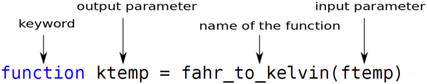
function ktemp = fahr_to_kelvin(ftemp)
    %FAHR_TO_KELVIN   Convert Fahrenheit to Kelvin

    ktemp = ((ftemp - 32) * (5/9)) + 273.15;
end

A MATLAB function must be saved in a text file with a .m extension. The name of that file must be the same as the function defined inside it. The name must start with a letter and cannot contain spaces. So, you will need to save the above code in a file called fahr_to_kelvin.m. Remember to save your m-files in the current directory.

The first line of our function is called the function definition, and it declares that we’re writing a function named fahr_to_kelvin, that has a single input parameter,ftemp, and a single output parameter, ktemp. Anything following the function definition line is called the body of the function. The keyword end marks the end of the function body, and the function won’t know about any code after end.

A function can have multiple input and output parameters if required, but isn’t required to have any of either. The general form of a function is shown in the pseudo-code below:

MATLAB

function [out1, out2] = function_name(in1, in2)
    %FUNCTION_NAME   Function description

    % This section below is called the body of the function
    out1 = something calculated;
    out2 = something else;
end

Just as we saw with scripts, functions must be visible to MATLAB, i.e., a file containing a function has to be placed in a directory that MATLAB knows about. The most convenient of those directories is the current working directory.

GNU Octave

In common with MATLAB, Octave searches the current working directory and the path for functions called from the command line.

We can call our function from the command line like any other MATLAB function:

MATLAB

>> fahr_to_kelvin(32)

OUTPUT

ans = 273.15

When we pass a value, like 32, to the function, the value is assigned to the variable ftemp so that it can be used inside the function. If we want to return a value from the function, we must assign that value to a variable named ktemp-–in the first line of our function, we promised that the output of our function would be named ktemp.

Outside of the function, the variables ftemp and ktemp aren’t visible; they are only used by the function body to refer to the input and output values.

This is one of the major differences between scripts and functions: a script can be thought of as automating the command line, with full access to all variables in the base workspace, whereas a function can only read and write variables from the calling workspace if they are passed as arguments — i.e. a function has its own separate workspace.

Now that we’ve seen how to convert Fahrenheit to Kelvin, it’s easy to convert Kelvin to Celsius.

MATLAB

function ctemp = kelvin_to_celsius(ktemp)
    %KELVIN_TO_CELSIUS   Convert from Kelvin to Celcius

    ctemp = ktemp - 273.15;
end

Again, we can call this function like any other:

MATLAB

>> kelvin_to_celsius(0.0)

OUTPUT

ans = -273.15

What about converting Fahrenheit to Celsius? We could write out the formula, but we don’t need to. Instead, we can compose the two functions we have already created:

MATLAB

function ctemp = fahr_to_celsius(ftemp)
    %FAHR_TO_CELSIUS   Convert Fahrenheit to Celcius

    ktemp = fahr_to_kelvin(ftemp);
    ctemp = kelvin_to_celsius(ktemp);
end

Calling this function,

MATLAB

>> fahr_to_celsius(32.0)

we get, as expected:

OUTPUT

ans = 0

This is our first taste of how larger programs are built: we define basic operations, then combine them in ever-larger chunks to get the effect we want. Real-life functions will usually be larger than the ones shown here—typically half a dozen to a few dozen lines—but they shouldn’t ever be much longer than that, or the next person who reads it won’t be able to understand what’s going on.

Concatenating in a Function

In MATLAB, we concatenate strings by putting them into an array or using the strcat function:

MATLAB

>> disp(['abra', 'cad', 'abra'])

OUTPUT

abracadabra

MATLAB

>> disp(strcat('a', 'b'))

OUTPUT

ab

Write a function called fence that has two parameters, original and wrapper and adds wrapper before and after original:

MATLAB

>> disp(fence('name', '*'))

OUTPUT

*name*

Show me the solution

MATLAB

function wrapped = fence(original, wrapper)
    %FENCE   Return original string, with wrapper prepended and appended

    wrapped = strcat(wrapper, original, wrapper);
end

Getting the Outside

If the variable s refers to a string, then s(1) is the string’s first character and s(end) is its last. Write a function called outer that returns a string made up of just the first and last characters of its input:

MATLAB

>> disp(outer('helium'))

OUTPUT

hm

Show me the solution

MATLAB

function ends = outer(s)
    %OUTER   Return first and last characters from a string

    ends = strcat(s(1), s(end));
end

Variables Inside and Outside Functions

Consider our function fahr_to_kelvin from earlier in the episode:

MATLAB

function ktemp = fahr_to_kelvin(ftemp)
  %FAHR_TO_KELVIN   Convert Fahrenheit to Kelvin
  ktemp = ((ftemp-32)*(5.0/9.0)) + 273.15;
end

What does the following code display when run — and why?

MATLAB

ftemp = 0
ktemp = 0

disp(fahr_to_kelvin(8))
disp(fahr_to_kelvin(41))
disp(fahr_to_kelvin(32))

disp(ktemp)

Show me the solution

OUTPUT

ktemp is 0 because the function fahr_to_kelvin has no knowledge of the variable ktemp which exists outside of the function.

Once we start putting things in functions so that we can re-use them, we need to start testing that those functions are working correctly. To see how to do this, let’s write a function to center a dataset around a particular value:

MATLAB

function out = center(data, desired)
    out = (data - mean(data(:))) + desired;
end

We could test this on our actual data, but since we don’t know what the values ought to be, it will be hard to tell if the result was correct, Instead, let’s create a matrix of 0’s, and then center that around 3:

MATLAB

>> z = zeros(2,2);
>> center(z, 3)

OUTPUT

That looks right, so let’s try out center function on our real data:

MATLAB

>> data = readmatrix('data/inflammation-01.csv');
>> centered = center(data(:), 0)

It’s hard to tell from the default output whether the result is correct–this is often the case when working with fairly large arrays–but, there are a few simple tests that will reassure us.

Let’s calculate some simple statistics:

MATLAB

>> disp([min(data(:)), mean(data(:)), max(data(:))])

OUTPUT

0.00000    6.14875   20.00000

And let’s do the same after applying our center function to the data:

MATLAB

>> disp([min(centered(:)), mean(centered(:)), max(centered(:))])

OUTPUT

   -6.1487   -0.0000   13.8513

That seems almost right: the original mean was about 6.1, so the lower bound from zero is now about -6.1. The mean of the centered data isn’t quite zero–we’ll explore why not in the challenges–but it’s pretty close. We can even go further and check that the standard deviation hasn’t changed:

MATLAB

>> std(data(:)) - std(centered(:))

OUTPUT

5.3291e-15

The difference is very small. It’s still possible that our function is wrong, but it seems unlikely enough that we should probably get back to doing our analysis. We have one more task first, though: we should write some documentation for our function to remind ourselves later what it’s for and how to use it.

MATLAB

function out = center(data, desired)
    %CENTER   Center data around a desired value.
    %
    %       center(DATA, DESIRED)
    %
    %   Returns a new array containing the values in
    %   DATA centered around the value.

    out = (data  - mean(data(:))) + desired;
end

Comment lines immediately below the function definition line are called “help text”. Typing help function_name brings up the help text for that function:

MATLAB

>> help center

OUTPUT

Center   Center data around a desired value.

    center(DATA, DESIRED)

Returns a new array containing the values in
DATA centered around the value.

Testing a Function

Write a function called normalise that takes an array as input and returns an array of the same shape with its values scaled to lie in the range 0.0 to 1.0. (If L and H are the lowest and highest values in the input array, respectively, then the function should map a value v to (v - L)/(H - L).) Be sure to give the function a comment block explaining its use.
Run help linspace to see how to use linspace to generate regularly-spaced values. Use arrays like this to test your normalise function.

Show me the solution

```
function out = normalise(in)
    %NORMALISE   Return original array, normalised so that the
    %            new values lie in the range 0 to 1.

    H = max(max(in));
    L = min(min(in));
    out = (in-L)/(H-L);
end
```
{: .language-matlab}

```
a = linspace(1, 10);   % Create evenly-spaced vector
norm_a = normalise(a); % Normalise vector
plot(a, norm_a)        % Visually check normalisation
```
{: .language-matlab}

Convert a script into a function

Write a function called plot_dataset which plots the three summary graphs (max, min, std) for a given inflammation data file.

The function should operate on a single data file, and should have two parameters: file_name and plot_switch. When called, the function should create the three graphs produced in the previous lesson. Whether they are displayed or saved to the results directory should be controlled by the value of plot_switch i.e. plot_dataset('data/inflammation-01.csv', 0) should display the corresponding graphs for the first data set; plot_dataset('data/inflammation-02.csv', 1) should save the figures for the second dataset to the results directory.

You should mostly be reusing code from the plot_all script.

Be sure to give your function help text.

Show me the solution

MATLAB

function plot_dataset(file_name, plot_switch)
    %PLOT_DATASET    Perform analysis for named data file.
    %   Create figures to show average, max and min inflammation.
    %   Display plots in GUI using plot_switch = 0,
    %   or save to disk using plot_switch = 1.
    %
    %   Example:
    %       plot_dataset('data/inflammation-01.csv', 0)
    
    % Generate string for image name:
    img_name = replace(file_name, '.csv', '.png');
    img_name = replace(img_name, 'data', 'results');

    patient_data = readmatrix(file_name);
    
    if plot_switch == 1
    	figure('visible', 'off')
    else
    	figure('visible', 'on')
    end
    
    subplot(2, 2, 1)
    plot(mean(patient_data, 1))
    ylabel('average')
    
    subplot(2, 2, 2)
    plot(max(patient_data, [], 1))
    ylabel('max')
    
    subplot(2, 2, 3)
    plot(min(patient_data, [], 1))
    ylabel('min')
    
    if plot_switch == 1
        print(img_name, '-dpng')
        close()
    end
 end

Automate the analysis for all files

Modify the plot_all script so that as it loops over the data files, it calls the function plot_dataset for each file in turn. Your script should save the image files to the ‘results’ directory rather than displaying the figures in the MATLAB GUI.

Show me the solution

MATLAB

%PLOT_ALL    Analyse all inflammation datasets
%   Create figures to show average, max and min inflammation.
%   Save figures to 'results' directory.

files = dir('data/inflammation-*.csv');

for i = 1:length(files)
    file_name = files(i).name;
    file_name = fullfile('data', file_name);

    % Process each data set, saving figures to disk.
    plot_dataset(file_name, 1);
end

We have now solved our original problem: we can analyze any number of data files with a single command. More importantly, we have met two of the most important ideas in programming:

Use arrays to store related values, and loops to repeat operations on them.
Use functions to make code easier to re-use and easier to understand.

Key Points

Break programs up into short, single-purpose functions with meaningful names.
Define functions using the function keyword.