Producing Reports With knitr
Last updated on 2024-04-04 | Edit this page
Overview
Questions
- How can I integrate software and reports?
Objectives
- Understand the value of writing reproducible reports
- Learn how to recognise and compile the basic components of an R Markdown file
- Become familiar with R code chunks, and understand their purpose, structure and options
- Demonstrate the use of inline chunks for weaving R outputs into text blocks, for example when discussing the results of some calculations
- Be aware of alternative output formats to which an R Markdown file can be exported
Data analysis reports
Data analysts tend to write a lot of reports, describing their analyses and results, for their collaborators or to document their work for future reference.
Many new users begin by first writing a single R script containing all of their work, and then share the analysis by emailing the script and various graphs as attachments. But this can be cumbersome, requiring a lengthy discussion to explain which attachment was which result.
Writing formal reports with Word or LaTeX can simplify this process by incorporating both the analysis report and output graphs into a single document. But tweaking formatting to make figures look correct and fixing obnoxious page breaks can be tedious and lead to a lengthy “whack-a-mole” game of fixing new mistakes resulting from a single formatting change.
Creating a report as a web page (which is an html file) using R Markdown makes things easier. The report can be one long stream, so tall figures that wouldn’t ordinarily fit on one page can be kept at full size and easier to read, since the reader can simply keep scrolling. Additionally, the formatting of and R Markdown document is simple and easy to modify, allowing you to spend more time on your analyses instead of writing reports.
Literate programming
Ideally, such analysis reports are reproducible documents: If an error is discovered, or if some additional subjects are added to the data, you can just re-compile the report and get the new or corrected results rather than having to reconstruct figures, paste them into a Word document, and hand-edit various detailed results.
The key R package here is knitr. It allows you
to create a document that is a mixture of text and chunks of code. When
the document is processed by knitr, chunks of code will be
executed, and graphs or other results will be inserted into the final
document.
This sort of idea has been called “literate programming”.
knitr allows you to mix basically any type of text with
code from different programming languages, but we recommend that you use
R Markdown, which mixes Markdown with R. Markdown is a light-weight
mark-up language for creating web pages.
Creating an R Markdown file
Within RStudio, click File → New File → R Markdown and you’ll get a dialog box like this:
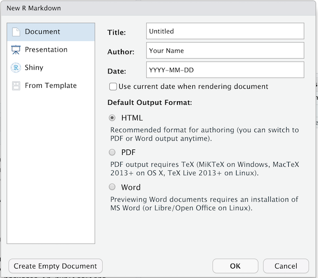
You can stick with the default (HTML output), but give it a title.
Basic components of R Markdown
The initial chunk of text (header) contains instructions for R to specify what kind of document will be created, and the options chosen. You can use the header to give your document a title, author, date, and tell it what type of output you want to produce. In this case, we’re creating an html document.
---
title: "Initial R Markdown document"
author: "Karl Broman"
date: "April 23, 2015"
output: html_document
---
You can delete any of those fields if you don’t want them included. The double-quotes aren’t strictly necessary in this case. They’re mostly needed if you want to include a colon in the title.
RStudio creates the document with some example text to get you started. Note below that there are chunks like
```{r}
summary(cars)
```
These are chunks of R code that will be executed by
knitr and replaced by their results. More on this
later.
Markdown
Markdown is a system for writing web pages by marking up the text much as you would in an email rather than writing html code. The marked-up text gets converted to html, replacing the marks with the proper html code.
For now, let’s delete all of the stuff that’s there and write a bit of markdown.
You make things bold using two asterisks, like this:
**bold**, and you make things italics by using
underscores, like this: _italics_.
You can make a bulleted list by writing a list with hyphens or asterisks with a space between the list and other text, like this:
A list:

* bold with double-asterisks
* italics with underscores
* code-type font with backticks
or like this:
A second list:

- bold with double-asterisks
- italics with underscores
- code-type font with backticks
Each will appear as:
- bold with double-asterisks
- italics with underscores
- code-type font with backticks
You can use whatever method you prefer, but be consistent. This maintains the readability of your code.
You can make a numbered list by just using numbers. You can even use the same number over and over if you want:
1. bold with double-asterisks
1. italics with underscores
1. code-type font with backticks
This will appear as:
- bold with double-asterisks
- italics with underscores
- code-type font with backticks
You can make section headers of different sizes by initiating a line
with some number of # symbols:
# Title
## Main section
### Sub-section
#### Sub-sub section
You compile the R Markdown document to an html webpage by clicking the “Knit” button in the upper-left.
In RStudio, select File > New file > R Markdown…
Delete the placeholder text and add the following:
# Introduction

## Background on Data

This report uses the *gapminder* dataset, which has columns that include:

* country
* continent
* year
* lifeExp
* pop
* gdpPercap

## Background on Methods
Then click the ‘Knit’ button on the toolbar to generate an html document (webpage).
A bit more Markdown
You can make a hyperlink like this:
[Carpentries Home Page](https://carpentries.org/).
You can include an image file like this:

You can do subscripts (e.g., F2) with F~2~
and superscripts (e.g., F2) with F^2^.
If you know how to write equations in LaTeX, you can use
$ $ and $$ $$ to insert math equations, like
$E = mc^2$ and
$$y = \mu + \sum_{i=1}^p \beta_i x_i + \epsilon$$You can review Markdown syntax by navigating to the “Markdown Quick Reference” under the “Help” field in the toolbar at the top of RStudio.
R code chunks
The real power of Markdown comes from mixing markdown with chunks of code. This is R Markdown. When processed, the R code will be executed; if they produce figures, the figures will be inserted in the final document.
The main code chunks look like this:
```{r load_data}
gapminder
That is, you place a chunk of R code between ```{r
chunk_name} and ```. You should give each chunk a
unique name, as they will help you to fix errors and, if any graphs are
produced, the file names are based on the name of the code chunk that
produced them. You can create code chunks quickly in RStudio using the
shortcuts Ctrl+Alt+I on Windows and
Linux, or Cmd+Option+I on Mac.
```{r load-ggplot2}
library("ggplot2")
```
```{r read-gapminder-data}
gapminder
```{r make-plot}
plot(lifeExp ~ year, data = gapminder)
```
How things get compiled
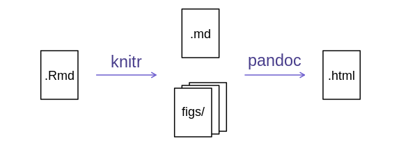
When you press the “Knit” button, the R Markdown document is
processed by knitr
and a plain Markdown document is produced (as well as, potentially, a
set of figure files): the R code is executed and replaced by both the
input and the output; if figures are produced, links to those figures
are included.
The Markdown and figure documents are then processed by the tool pandoc, which converts the
Markdown file into an html file, with the figures embedded.
Chunk options
There are a variety of options to affect how the code chunks are treated. Here are some examples:
- Use
echo=FALSEto avoid having the code itself shown. - Use
results="hide"to avoid having any results printed. - Use
eval=FALSEto have the code shown but not evaluated. - Use
warning=FALSEandmessage=FALSEto hide any warnings or messages produced. - Use
fig.heightandfig.widthto control the size of the figures produced (in inches).
So you might write:
```{r load_libraries, echo=FALSE, message=FALSE}
library("dplyr")
library("ggplot2")
```
Often there will be particular options that you’ll want to use repeatedly; for this, you can set global chunk options, like so:
```{r global_options, echo=FALSE}
knitr::opts_chunk$set(fig.path="Figs/", message=FALSE, warning=FALSE,
                      echo=FALSE, results="hide", fig.width=11)
```
The fig.path option defines where the figures will be
saved. The / here is really important; without it, the
figures would be saved in the standard place but just with names that
begin with Figs.
If you have multiple R Markdown files in a common directory, you
might want to use fig.path to define separate prefixes for
the figure file names, like fig.path="Figs/cleaning-" and
fig.path="Figs/analysis-".
```{r echo = FALSE, fig.width = 3}
plot(faithful)
```
You can review all of the R chunk options by navigating
to the “R Markdown Cheat Sheet” under the “Cheatsheets” section of the
“Help” field in the toolbar at the top of RStudio.
Inline R code
You can make every number in your report reproducible. Use
`r and ` for an in-line code chunk, like so:
`r round(some_value, 2)`. The code will be executed and
replaced with the value of the result.
Don’t let these in-line chunks get split across lines.
Perhaps precede the paragraph with a larger code chunk that does
calculations and defines variables, with include=FALSE for
that larger chunk (which is the same as echo=FALSE and
results="hide").
Rounding can produce differences in output in such situations. You
may want 2.0, but round(2.03, 1) will give
just 2.
The myround
function in the R/broman
package handles this.
Here’s some inline code to determine that 2 + 2 = 4.
Other output options
You can also convert R Markdown to a PDF or a Word document. Click
the little triangle next to the “Knit” button to get a drop-down menu.
Or you could put pdf_document or word_document
in the initial header of the file.
Tip: Creating PDF documents
Creating .pdf documents may require installation of some extra
software. The R package tinytex provides some tools to help
make this process easier for R users. With tinytex
installed, run tinytex::install_tinytex() to install the
required software (you’ll only need to do this once) and then when you
knit to pdf tinytex will automatically detect and install
any additional LaTeX packages that are needed to produce the pdf
document. Visit the tinytex
website for more information.
Tip: Visual markdown editing in RStudio
RStudio versions 1.4 and later include visual markdown editing mode.
In visual editing mode, markdown expressions (like
**bold words**) are transformed to the formatted appearance
(bold words) as you type. This mode also includes a
toolbar at the top with basic formatting buttons, similar to what you
might see in common word processing software programs. You can turn
visual editing on and off by pressing the ![]() button in the top right corner of your R Markdown document.
button in the top right corner of your R Markdown document.