Overview
Teaching: 20 min
Exercises: 0 minQuestions
What are the different methods for accessing parts of a data frame?
Objectives
Understand the three different ways R can address data inside a data frame.
Combine different methods for addressing data with the assignment operator to update subsets of data.
R is a powerful language for data manipulation. There are three main ways for addressing data inside R objects.
- By index (slicing)
- By logical vector
- By name (columns only)
Lets start by loading some sample data:
dat <- read.csv(file = 'data/sample.csv', header = TRUE, stringsAsFactors = FALSE)
Interpreting Rows as Headers
The first row of this csv file is a list of column names. We used the header=TRUE argument to
read.csvso that R can interpret the file correctly. We are using the stringsAsFactors=FALSE argument to override the default behaviour for R. Using factors in R is covered in a separate lesson.
Lets take a look at this data.
class(dat)
[1] "data.frame"
R has loaded the contents of the .csv file into a variable called dat which is a data frame.
dim(dat)
[1] 100 9
The data has 100 rows and 9 columns.
head(dat)
      ID Gender      Group BloodPressure  Age Aneurisms_q1 Aneurisms_q2
1 Sub001      m    Control           132 16.0          114          140
2 Sub002      m Treatment2           139 17.2          148          209
3 Sub003      m Treatment2           130 19.5          196          251
4 Sub004      f Treatment1           105 15.7          199          140
5 Sub005      m Treatment1           125 19.9          188          120
6 Sub006      M Treatment2           112 14.3          260          266
  Aneurisms_q3 Aneurisms_q4
1          202          237
2          248          248
3          122          177
4          233          220
5          222          228
6          320          294
The data is the results of an (not real) experiment, looking at the number of aneurysms that formed in the eyes of patients who undertook 3 different treatments.
Addressing by Index
Data can be accessed by index. We have already seen how square brackets [ can be used to subset (slice) data. The generic format is dat[row_numbers,column_numbers].
Selecting Values
What will be returned by
dat[1,1]?
dat[1,1]
[1] "Sub001"
If we leave out a dimension R will interpret this as a request for all values in that dimension.
Selecting More Values
What will be returned by
dat[,2]?
The colon : can be used to create a sequence of integers.
6:9
[1] 6 7 8 9
Creates a vector of numbers from 6 to 9.
This can be very useful for addressing data.
Subsetting with Sequences
Use the colon operator to index just the aneurism count data (columns 6 to 9).
Finally we can use the c() (combine) function to address non-sequential rows and columns.
dat[c(1,5,7,9), 1:5]
      ID Gender      Group BloodPressure  Age
1 Sub001      m    Control           132 16.0
5 Sub005      m Treatment1           125 19.9
7 Sub007      f    Control           173 17.7
9 Sub009      m Treatment2           131 19.4
Returns the first 5 columns for patients in rows 1,5,7 & 9
Subsetting Non-Sequential Data
Return the age and gender values for the first 5 patients.
Addressing by Name
Columns in an R data frame are named.
names(dat)
[1] "ID"            "Gender"        "Group"         "BloodPressure"
[5] "Age"           "Aneurisms_q1"  "Aneurisms_q2"  "Aneurisms_q3"
[9] "Aneurisms_q4"
Default Names
If names are not specified e.g. using
headers=FALSEin aread.csv()function, R assigns default namesV1,V2,...,Vn
We usually use the $ operator to address a column by name
dat$Gender
  [1] "m" "m" "m" "f" "m" "M" "f" "m" "m" "f" "m" "f" "f" "m" "m" "m" "f"
 [18] "m" "m" "F" "f" "m" "f" "f" "m" "M" "M" "f" "m" "f" "f" "m" "m" "m"
 [35] "m" "f" "f" "m" "M" "m" "f" "m" "m" "m" "f" "f" "M" "M" "m" "m" "m"
 [52] "f" "f" "f" "m" "f" "m" "m" "m" "f" "f" "f" "f" "M" "f" "m" "f" "f"
 [69] "M" "m" "m" "m" "F" "m" "m" "f" "M" "M" "M" "f" "m" "M" "M" "m" "m"
 [86] "f" "f" "f" "m" "m" "f" "m" "F" "f" "m" "m" "F" "m" "M" "M"
Named addressing can also be used in square brackets.
head(dat[,c('Age', 'Gender')])
   Age Gender
1 16.0      m
2 17.2      m
3 19.5      m
4 15.7      f
5 19.9      m
6 14.3      M
Best Practice
Best practice is to address columns by name, often you will create or delete columns and the column position will change.
Logical Indexing
A logical vector contains only the special values TRUE & FALSE.
c(TRUE, TRUE, FALSE, FALSE, TRUE)
[1] TRUE TRUE FALSE FALSE TRUE
Truth and Its Opposite
Note the values
TRUEandFALSEare all capital letters and are not quoted.
Logical vectors can be created using relational operators e.g. <, >, ==, !=, %in%.
x <- c(1, 2, 3, 11, 12, 13)
x < 10
[1] TRUE TRUE TRUE FALSE FALSE FALSE
x %in% 1:10
[1] TRUE TRUE TRUE FALSE FALSE FALSE
We can use logical vectors to select data from a data frame.
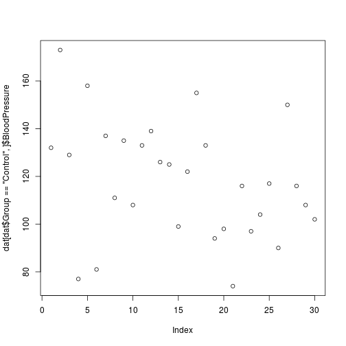
index <- dat$Group == 'Control'
dat[index,]$BloodPressure
 [1] 132 173 129  77 158  81 137 111 135 108 133 139 126 125  99 122 155
[18] 133  94  98  74 116  97 104 117  90 150 116 108 102
Often this operation is written as one line of code:
plot(dat[dat$Group == 'Control',]$BloodPressure)

Using Logical Indexes
- Create a scatterplot showing BloodPressure for subjects not in the control group.
- How many ways are there to index this set of subjects?
Combining Indexing and Assignment
The assignment operator <- can be combined with indexing.
x <- c(1, 2, 3, 11, 12, 13)
x[x < 10] <- 0
x
[1] 0 0 0 11 12 13
Updating a Subset of Values
In this dataset, values for Gender have been recorded as both uppercase
M, Fand lowercasem,f. Combine the indexing and assignment operations to convert all values to lowercase.
Key Points
Data in data frames can be addressed by index (slicing), by logical vector, or by name (columns only).
Use the
$operator to address a column by name.