All in One View
Content from Selecting Data
Last updated on 2026-01-27 | Edit this page
Overview
Questions
- How can I get data from a database?
Objectives
- Explain the difference between a table, a record, and a field.
- Explain the difference between a database and a database manager.
- Write a query to select all values for specific fields from a single table.
A relational database is a way to store and manipulate information. Databases are arranged as tables. Each table has columns (also known as fields) that describe the data, and rows (also known as records) which contain the data.

When we are using a spreadsheet, we put formulas into cells to calculate new values based on old ones. When we are using a database, we send commands (usually called queries to a database manager: a program that manipulates the database for us. The database manager does whatever lookups and calculations the query specifies, returning the results in a tabular form that we can then use as a starting point for further queries.
Queries are written in a language called SQL, which stands for “Structured Query Language”. SQL provides hundreds of different ways to analyze and recombine data. We will only look at a handful of queries, but that handful accounts for most of what scientists do.
Changing Database Managers
Many database managers — Oracle, IBM DB2, PostgreSQL, MySQL, Microsoft Access, and SQLite — understand SQL but each stores data in a different way, so a database created with one cannot be used directly by another. However, every database manager can import and export data in a variety of formats like .csv, SQL, so it is possible to move information from one to another.
Getting Into and Out Of SQLite
In order to use the SQLite commands interactively, we need to enter into the SQLite console. So, open up a terminal, and run
The SQLite command is sqlite3 and you are telling SQLite
to open up the survey.db. You need to specify the
.db file, otherwise SQLite will open up a temporary, empty
database.
To get out of SQLite, type out .exit or
.quit. For some terminals, Ctrl-D can also
work. If you forget any SQLite . (dot) command, type
.help.
Before we get into using SQLite to select the data, let’s take a look at the tables of the database we will use in our examples:
Person: People who took readings, id
being the unique identifier for that person.
| id | personal | family |
|---|---|---|
| dyer | William | Dyer |
| pb | Frank | Pabodie |
| lake | Anderson | Lake |
| roe | Valentina | Roerich |
| danforth | Frank | Danforth |
Site: Locations of the sites where
readings were taken.
| name | lat | long |
|---|---|---|
| DR-1 | -49.85 | -128.57 |
| DR-3 | -47.15 | -126.72 |
| MSK-4 | -48.87 | -123.4 |
Visited: Specific identification id of
the precise locations where readings were taken at the sites and
dates.
| id | site | dated |
|---|---|---|
| 619 | DR-1 | 1927-02-08 |
| 622 | DR-1 | 1927-02-10 |
| 734 | DR-3 | 1930-01-07 |
| 735 | DR-3 | 1930-01-12 |
| 751 | DR-3 | 1930-02-26 |
| 752 | DR-3 | -null- |
| 837 | MSK-4 | 1932-01-14 |
| 844 | DR-1 | 1932-03-22 |
Survey: The measurements taken at each precise
location on these sites. They are identified as taken. The
field quant is short for quantity and indicates what is
being measured. The values are rad, sal, and
temp referring to ‘radiation’, ‘salinity’ and
‘temperature’, respectively.
| taken | person | quant | reading |
|---|---|---|---|
| 619 | dyer | rad | 9.82 |
| 619 | dyer | sal | 0.13 |
| 622 | dyer | rad | 7.8 |
| 622 | dyer | sal | 0.09 |
| 734 | pb | rad | 8.41 |
| 734 | lake | sal | 0.05 |
| 734 | pb | temp | -21.5 |
| 735 | pb | rad | 7.22 |
| 735 | -null- | sal | 0.06 |
| 735 | -null- | temp | -26.0 |
| 751 | pb | rad | 4.35 |
| 751 | pb | temp | -18.5 |
| 751 | lake | sal | 0.1 |
| 752 | lake | rad | 2.19 |
| 752 | lake | sal | 0.09 |
| 752 | lake | temp | -16.0 |
| 752 | roe | sal | 41.6 |
| 837 | lake | rad | 1.46 |
| 837 | lake | sal | 0.21 |
| 837 | roe | sal | 22.5 |
| 844 | roe | rad | 11.25 |
Notice that three entries — one in the Visited table,
and two in the Survey table — don’t contain any actual
data, but instead have a special -null- entry: we’ll return
to these missing values later.
Checking If Data is Available
On the shell command line, change the working directory to the one
where you saved survey.db. If you saved it at your Desktop
you should use
OUTPUT
survey.dbIf you get the same output, you can run
OUTPUT
SQLite version 3.8.8 2015-01-16 12:08:06
Enter ".help" for usage hints.
sqlite>
that instructs SQLite to load the database in the
survey.db file.
For a list of useful system commands, enter .help.
All SQLite-specific commands are prefixed with a . to
distinguish them from SQL commands.
Type .tables to list the tables in the database.
OUTPUT
Person Site Survey VisitedIf you had the above tables, you might be curious what information
was stored in each table. To get more information on the tables, type
.schema to see the SQL statements used to create the tables
in the database. The statements will have a list of the columns and the
data types each column stores.
OUTPUT
CREATE TABLE Person (id text, personal text, family text);
CREATE TABLE Site (name text, lat real, long real);
CREATE TABLE Survey (taken integer, person text, quant text, reading real);
CREATE TABLE Visited (id integer, site text, dated text);
The output is formatted as <columnName dataType>. Thus we can see from the first line that the table Person has three columns:
- id with type text
- personal with type text
- family with type text
Note: The available data types vary based on the database manager - you can search online for what data types are supported.
You can change some SQLite settings to make the output easier to read. First, set the output mode to display left-aligned columns. Then turn on the display of column headers.
Alternatively, you can get the settings automatically by creating a
.sqliterc file. Add the commands above and reopen SQLite.
For Windows, use C:\Users\<yourusername>.sqliterc.
For Linux/MacOS, use
/Users/<yourusername>/.sqliterc.
To exit SQLite and return to the shell command line, you can use
either .quit or .exit.
For now, let’s write an SQL query that displays scientists’ names. We
do this using the SQL command SELECT, giving it the names
of the columns we want and the table we want them from. Our query and
its output, with the above settings applied, look like this:
| family | personal |
|---|---|
| Dyer | William |
| Pabodie | Frank |
| Lake | Anderson |
| Roerich | Valentina |
| Danforth | Frank |
The semicolon at the end of the query tells the database manager that the query is complete and ready to run.
For comparison, without the above settings, the output of the same query will look like this:
William|Dyer
Frank|Pabodie
Anderson|Lake
Valentina|Roerich
Frank|Danforth
We have written our commands in upper case and the names for the table and columns in lower case, but we don’t have to: as the example below shows, SQL is case insensitive.
| family | personal |
|---|---|
| Dyer | William |
| Pabodie | Frank |
| Lake | Anderson |
| Roerich | Valentina |
| Danforth | Frank |
You can use SQL’s case insensitivity to distinguish between different
parts of an SQL statement. In this lesson, we use the convention of
using UPPER CASE for SQL keywords (such as SELECT and
FROM), Title Case for table names, and lower case for field
names. Whatever casing convention you choose, please be consistent:
complex queries are hard enough to read without the extra cognitive load
of random capitalization.
While we are on the topic of SQL’s syntax, one aspect of SQL’s syntax
that can frustrate novices and experts alike is forgetting to finish a
command with ; (semicolon). When you press enter for a
command without adding the ; to the end, it can look
something like this:
This is SQL’s prompt, where it is waiting for additional commands or
for a ; to let SQL know to finish. This is easy to fix!
Just type ; and press enter!
Now, going back to our query, it’s important to understand that the rows and columns in a database table aren’t actually stored in any particular order. They will always be displayed in some order, but we can control that in various ways. For example, we could swap the columns in the output by writing our query as:
| personal | family |
|---|---|
| William | Dyer |
| Frank | Pabodie |
| Anderson | Lake |
| Valentina | Roerich |
| Frank | Danforth |
or even repeat columns:
| id | id | id |
|---|---|---|
| dyer | dyer | dyer |
| pb | pb | pb |
| lake | lake | lake |
| roe | roe | roe |
| danforth | danforth | danforth |
As a shortcut, we can select all of the columns in a table using
*:
| id | personal | family |
|---|---|---|
| dyer | William | Dyer |
| pb | Frank | Pabodie |
| lake | Anderson | Lake |
| roe | Valentina | Roerich |
| danforth | Frank | Danforth |
Understanding CREATE statements
Use the .schema to identify column that contains
integers.
OUTPUT
CREATE TABLE Person (id text, personal text, family text);
CREATE TABLE Site (name text, lat real, long real);
CREATE TABLE Survey (taken integer, person text, quant text, reading real);
CREATE TABLE Visited (id integer, site text, dated text);
From the output, we see that the taken column in the Survey table (3rd line) is composed of integers.
Selecting Site Names
Write a query that selects only the name column from the
Site table.
- A relational database stores information in tables, each of which has a fixed set of columns and a variable number of records.
- A database manager is a program that manipulates information stored in a database.
- We write queries in a specialized language called SQL to extract information from databases.
- Use SELECT… FROM… to get values from a database table.
- SQL is case-insensitive (but data is case-sensitive).
Content from Sorting and Removing Duplicates
Last updated on 2023-05-08 | Edit this page
Overview
Questions
- How can I sort a query’s results?
- How can I remove duplicate values from a query’s results?
Objectives
- Write queries that display results in a particular order.
- Write queries that eliminate duplicate values from data.
In beginning our examination of the Antarctic data, we want to know:
- what kind of quantity measurements were taken at each site;
- which scientists took measurements on the expedition;
To determine which measurements were taken at each site, we can
examine the Survey table. Data is often redundant, so
queries often return redundant information. For example, if we select
the quantities that have been measured from the Survey
table, we get this:
| quant |
|---|
| rad |
| sal |
| rad |
| sal |
| rad |
| sal |
| temp |
| rad |
| sal |
| temp |
| rad |
| temp |
| sal |
| rad |
| sal |
| temp |
| sal |
| rad |
| sal |
| sal |
| rad |
This result makes it difficult to see all of the different types of
quant in the Survey table. We can eliminate the redundant
output to make the result more readable by adding the
DISTINCT keyword to our query:
| quant |
|---|
| rad |
| sal |
| temp |
If we want to determine which visit (stored in the taken
column) have which quant measurement, we can use the
DISTINCT keyword on multiple columns. If we select more
than one column, distinct sets of values are returned (in this
case pairs, because we are selecting two columns):
| taken | quant |
|---|---|
| 619 | rad |
| 619 | sal |
| 622 | rad |
| 622 | sal |
| 734 | rad |
| 734 | sal |
| 734 | temp |
| 735 | rad |
| 735 | sal |
| 735 | temp |
| 751 | rad |
| 751 | temp |
| 751 | sal |
| 752 | rad |
| 752 | sal |
| 752 | temp |
| 837 | rad |
| 837 | sal |
| 844 | rad |
Notice in both cases that duplicates are removed even if the rows they come from didn’t appear to be adjacent in the database table.
Our next task is to identify the scientists on the expedition by
looking at the Person table. As we mentioned earlier,
database records are not stored in any particular order. This means that
query results aren’t necessarily sorted, and even if they are, we often
want to sort them in a different way, e.g., by their identifier instead
of by their personal name. We can do this in SQL by adding an
ORDER BY clause to our query:
| id | personal | family |
|---|---|---|
| danfort | Frank | Danforth |
| dyer | William | Dyer |
| lake | Anderson | Lake |
| pb | Frank | Pabodie |
| roe | Valentina | Roerich |
By default, when we use ORDER BY, results are sorted in
ascending order of the column we specify (i.e., from least to
greatest).
We can sort in the opposite order using DESC (for
“descending”):
A note on ordering
While it may look that the records are consistent every time we ask
for them in this lesson, that is because no one has changed or modified
any of the data so far. Remember to use ORDER BY if you
want the rows returned to have any sort of consistent or predictable
order.
| id | personal | family |
|---|---|---|
| roe | Valentina | Roerich |
| pb | Frank | Pabodie |
| lake | Anderson | Lake |
| dyer | William | Dyer |
| danfort | Frank | Danforth |
(And if we want to make it clear that we’re sorting in ascending
order, we can use ASC instead of DESC.)
In order to look at which scientist measured quantities during each
visit, we can look again at the Survey table. We can also
sort on several fields at once. For example, this query sorts results
first in ascending order by taken, and then in descending
order by person within each group of equal
taken values:
| taken | person | quant |
|---|---|---|
| 619 | dyer | rad |
| 619 | dyer | sal |
| 622 | dyer | rad |
| 622 | dyer | sal |
| 734 | pb | rad |
| 734 | pb | temp |
| 734 | lake | sal |
| 735 | pb | rad |
| 735 | -null- | sal |
| 735 | -null- | temp |
| 751 | pb | rad |
| 751 | pb | temp |
| 751 | lake | sal |
| 752 | roe | sal |
| 752 | lake | rad |
| 752 | lake | sal |
| 752 | lake | temp |
| 837 | roe | sal |
| 837 | lake | rad |
| 837 | lake | sal |
| 844 | roe | rad |
This query gives us a good idea of which scientist was involved in which visit, and what measurements they performed during the visit.
Looking at the table, it seems like some scientists specialized in certain kinds of measurements. We can examine which scientists performed which measurements by selecting the appropriate columns and removing duplicates.
| quant | person |
|---|---|
| rad | dyer |
| rad | pb |
| rad | lake |
| rad | roe |
| sal | dyer |
| sal | lake |
| sal | -null- |
| sal | roe |
| temp | pb |
| temp | -null- |
| temp | lake |
Finding Distinct Dates
Write a query that selects distinct dates from the
Visited table.
Displaying Full Names
Write a query that displays the full names of the scientists in the
Person table, ordered by family name.
- The records in a database table are not intrinsically ordered: if we want to display them in some order, we must specify that explicitly with ORDER BY.
- The values in a database are not guaranteed to be unique: if we want to eliminate duplicates, we must specify that explicitly as well using DISTINCT.
Content from Filtering
Last updated on 2023-05-08 | Edit this page
Overview
Questions
- How can I select subsets of data?
Objectives
- Write queries that select records that satisfy user-specified conditions.
- Explain the order in which the clauses in a query are executed.
One of the most powerful features of a database is the ability to filter data, i.e., to select only those
records that match certain criteria. For example, suppose we want to see
when a particular site was visited. We can select these records from the
Visited table by using a WHERE clause in our
query:
| id | site | dated |
|---|---|---|
| 619 | DR-1 | 1927-02-08 |
| 622 | DR-1 | 1927-02-10 |
| 844 | DR-1 | 1932-03-22 |
The database manager executes this query in two stages. First, it
checks at each row in the Visited table to see which ones
satisfy the WHERE. It then uses the column names following
the SELECT keyword to determine which columns to
display.
This processing order means that we can filter records using
WHERE based on values in columns that aren’t then
displayed:
| id |
|---|
| 619 |
| 622 |
| 844 |

We can use many other Boolean operators to filter our data. For example, we can ask for all information from the DR-1 site collected before 1930:
| id | site | dated |
|---|---|---|
| 619 | DR-1 | 1927-02-08 |
| 622 | DR-1 | 1927-02-10 |
Date Types
Most database managers have a special data type for dates. In fact, many have two: one for dates, such as “May 31, 1971”, and one for durations, such as “31 days”. SQLite doesn’t: instead, it stores dates as either text (in the ISO-8601 standard format “YYYY-MM-DD HH:MM:SS.SSSS”), real numbers (Julian days, the number of days since November 24, 4714 BCE), or integers (Unix time, the number of seconds since midnight, January 1, 1970). If this sounds complicated, it is, but not nearly as complicated as figuring out historical dates in Sweden.
If we want to find out what measurements were taken by either Lake or
Roerich, we can combine the tests on their names using
OR:
| taken | person | quant | reading |
|---|---|---|---|
| 734 | lake | sal | 0.05 |
| 751 | lake | sal | 0.1 |
| 752 | lake | rad | 2.19 |
| 752 | lake | sal | 0.09 |
| 752 | lake | temp | -16.0 |
| 752 | roe | sal | 41.6 |
| 837 | lake | rad | 1.46 |
| 837 | lake | sal | 0.21 |
| 837 | roe | sal | 22.5 |
| 844 | roe | rad | 11.25 |
Alternatively, we can use IN to see if a value is in a
specific set:
| taken | person | quant | reading |
|---|---|---|---|
| 734 | lake | sal | 0.05 |
| 751 | lake | sal | 0.1 |
| 752 | lake | rad | 2.19 |
| 752 | lake | sal | 0.09 |
| 752 | lake | temp | -16.0 |
| 752 | roe | sal | 41.6 |
| 837 | lake | rad | 1.46 |
| 837 | lake | sal | 0.21 |
| 837 | roe | sal | 22.5 |
| 844 | roe | rad | 11.25 |
We can combine AND with OR, but we need to
be careful about which operator is executed first. If we don’t
use parentheses, we get this:
| taken | person | quant | reading |
|---|---|---|---|
| 734 | lake | sal | 0.05 |
| 751 | lake | sal | 0.1 |
| 752 | lake | sal | 0.09 |
| 752 | roe | sal | 41.6 |
| 837 | lake | sal | 0.21 |
| 837 | roe | sal | 22.5 |
| 844 | roe | rad | 11.25 |
which is salinity measurements by Lake, and any measurement by Roerich. We probably want this instead:
| taken | person | quant | reading |
|---|---|---|---|
| 734 | lake | sal | 0.05 |
| 751 | lake | sal | 0.1 |
| 752 | lake | sal | 0.09 |
| 752 | roe | sal | 41.6 |
| 837 | lake | sal | 0.21 |
| 837 | roe | sal | 22.5 |
We can also filter by partial matches. For example, if we want to
know something just about the site names beginning with “DR” we can use
the LIKE keyword. The percent symbol acts as a wildcard, matching any characters in
that place. It can be used at the beginning, middle, or end of the
string:
| id | site | dated |
|---|---|---|
| 619 | DR-1 | 1927-02-08 |
| 622 | DR-1 | 1927-02-10 |
| 734 | DR-3 | 1930-01-07 |
| 735 | DR-3 | 1930-01-12 |
| 751 | DR-3 | 1930-02-26 |
| 752 | DR-3 | |
| 844 | DR-1 | 1932-03-22 |
Finally, we can use DISTINCT with WHERE to
give a second level of filtering:
| person | quant |
|---|---|
| lake | sal |
| lake | rad |
| lake | temp |
| roe | sal |
| roe | rad |
But remember: DISTINCT is applied to the values
displayed in the chosen columns, not to the entire rows as they are
being processed.
Growing Queries
What we have just done is how most people “grow” their SQL queries. We started with something simple that did part of what we wanted, then added more clauses one by one, testing their effects as we went. This is a good strategy — in fact, for complex queries it’s often the only strategy — but it depends on quick turnaround, and on us recognizing the right answer when we get it.
The best way to achieve a quick turnaround is often to put a subset of data in a temporary database and run our queries against that, or to fill a small database with synthesized records. For example, instead of trying our queries against an actual database of 20 million Australians, we could run it against a sample of ten thousand, or write a small program to generate ten thousand random (but plausible) records and use that.
Finding Outliers
Normalized salinity readings are supposed to be between 0.0 and 1.0.
Write a query that selects all records from Survey with
salinity values outside this range.
Matching Patterns
Which of these expressions are true?
'a' LIKE 'a''a' LIKE '%a''beta' LIKE '%a''alpha' LIKE 'a%%''alpha' LIKE 'a%p%'
- True because these are the same character.
- True because the wildcard can match zero or more characters.
- True because the
%matchesbetand theamatches thea. - True because the first wildcard matches
lphaand the second wildcard matches zero characters (or vice versa). - True because the first wildcard matches
land the second wildcard matchesha.
- Use WHERE to specify conditions that records must meet in order to be included in a query’s results.
- Use AND, OR, and NOT to combine tests.
- Filtering is done on whole records, so conditions can use fields that are not actually displayed.
- Write queries incrementally.
Content from Calculating New Values
Last updated on 2026-01-27 | Edit this page
Overview
Questions
- How can I calculate new values on the fly?
Objectives
- Write queries that calculate new values for each selected record.
After carefully re-reading the expedition logs, we realize that the radiation measurements they report may need to be corrected upward by 5%. Rather than modifying the stored data, we can do this calculation on the fly as part of our query:
| 1.05 * reading |
|---|
| 10.311 |
| 8.19 |
| 8.8305 |
| 7.581 |
| 4.5675 |
| 2.2995 |
| 1.533 |
| 11.8125 |
When we run the query, the expression 1.05 * reading is
evaluated for each row. Expressions can use any of the fields, all of
usual arithmetic operators, and a variety of common functions. (Exactly
which ones depends on which database manager is being used.) For
example, we can convert temperature readings from Fahrenheit to Celsius
and round to two decimal places:
| taken | round(5*(reading-32)/9, 2) |
|---|---|
| 734 | -29.72 |
| 735 | -32.22 |
| 751 | -28.06 |
| 752 | -26.67 |
As you can see from this example, though, the string describing our new field (generated from the equation) can become quite unwieldy. SQL allows us to rename our fields, any field for that matter, whether it was calculated or one of the existing fields in our database, for succinctness and clarity. For example, we could write the previous query as:
| taken | Celsius |
|---|---|
| 734 | -29.72 |
| 735 | -32.22 |
| 751 | -28.06 |
| 752 | -26.67 |
We can also combine values from different fields, for example by
using the string concatenation operator ||:
| personal |
|---|
| William Dyer |
| Frank Pabodie |
| Anderson Lake |
| Valentina Roerich |
| Frank Danforth |
Fixing Salinity Readings
After further reading, we realize that Valentina Roerich was
reporting salinity as percentages. Write a query that returns all of her
salinity measurements from the Survey table with the values
divided by 100.
Unions
The UNION operator combines the results of two
queries:
| id | personal | family |
|---|---|---|
| dyer | William | Dyer |
| roe | Valentina | Roerich |
The UNION ALL command is equivalent to the
UNION operator, except that UNION ALL will
select all values. The difference is that UNION ALL will
not eliminate duplicate rows. Instead, UNION ALL pulls all
rows from the query specifics and combines them into a table. The
UNION command does a SELECT DISTINCT on the
results set. If all the records to be returned are unique from your
union, use UNION ALL instead, it gives faster results since
it skips the DISTINCT step. For this section, we shall use
UNION.
Use UNION to create a consolidated list of salinity
measurements in which Valentina Roerich’s, and only Valentina’s, have
been corrected as described in the previous challenge. The output should
be something like:
| taken | reading |
|---|---|
| 619 | 0.13 |
| 622 | 0.09 |
| 734 | 0.05 |
| 751 | 0.1 |
| 752 | 0.09 |
| 752 | 0.416 |
| 837 | 0.21 |
| 837 | 0.225 |
Selecting Major Site Identifiers
The site identifiers in the Visited table have two parts
separated by a ‘-’:
| site |
|---|
| DR-1 |
| DR-3 |
| MSK-4 |
The sites are identified by a few letters, a dash, and a number.
Suppose you want to see what are the major sites where data has been
collected. In our data, those would be the sites denoted with the letter
codes such as DR or MSK. However, some major
site identifiers (i.e. the letter codes) are two letters long and some
are three. Therefore, we need to run some kind of operation on the site
string to be able to get just the letter codes.
SQLite has functions that would enable us to do just that. The “in
string” function instr(X, Y) returns the 1-based index of
the first occurrence of string Y in string X, or 0 if Y does not exist
in X. For example, the query:
Would return the position of the - character in each
site:
| indexes |
|---|
| 3 |
| 3 |
| 3 |
The substring function substr(X, I, [L]) returns the
substring of X starting at index I, with an optional length L. For
example, the query:
Would return the first letter of each site:
| first_char |
|---|
| D |
| D |
| D |
Combine these two functions to produce a list of unique major site identifiers. (For this data, the list should contain only “DR” and “MSK”).
- Queries can do the usual arithmetic operations on values.
- Use UNION to combine the results of two or more queries.
Content from Missing Data
Last updated on 2023-05-08 | Edit this page
Overview
Questions
- How do databases represent missing information?
- What special handling does missing information require?
Objectives
- Explain how databases represent missing information.
- Explain the three-valued logic databases use when manipulating missing information.
- Write queries that handle missing information correctly.
Real-world data is never complete — there are always holes. Databases
represent these holes using a special value called null.
null is not zero, False, or the empty string;
it is a one-of-a-kind value that means “nothing here”. Dealing with
null requires a few special tricks and some careful
thinking.
By default, SQLite does not display NULL values in its output. The
.nullvalue command causes SQLite to display the value you
specify for NULLs. We will use the value -null- to make the
NULLs easier to see:
To start, let’s have a look at the Visited table. There
are eight records, but #752 doesn’t have a date — or rather, its date is
null:
| id | site | dated |
|---|---|---|
| 619 | DR-1 | 1927-02-08 |
| 622 | DR-1 | 1927-02-10 |
| 734 | DR-3 | 1930-01-07 |
| 735 | DR-3 | 1930-01-12 |
| 751 | DR-3 | 1930-02-26 |
| 752 | DR-3 | -null- |
| 837 | MSK-4 | 1932-01-14 |
| 844 | DR-1 | 1932-03-22 |
Null doesn’t behave like other values. If we select the records that come before 1930:
| id | site | dated |
|---|---|---|
| 619 | DR-1 | 1927-02-08 |
| 622 | DR-1 | 1927-02-10 |
we get two results, and if we select the ones that come during or after 1930:
| id | site | dated |
|---|---|---|
| 734 | DR-3 | 1930-01-07 |
| 735 | DR-3 | 1930-01-12 |
| 751 | DR-3 | 1930-02-26 |
| 837 | MSK-4 | 1932-01-14 |
| 844 | DR-1 | 1932-03-22 |
we get five, but record #752 isn’t in either set of results. The
reason is that null<'1930-01-01' is neither true nor
false: null means, “We don’t know,” and if we don’t know the value on
the left side of a comparison, we don’t know whether the comparison is
true or false. Since databases represent “don’t know” as null, the value
of null<'1930-01-01' is actually null.
null>='1930-01-01' is also null because we can’t answer
to that question either. And since the only records kept by a
WHERE are those for which the test is true, record #752
isn’t included in either set of results.
Comparisons aren’t the only operations that behave this way with
nulls. 1+null is null, 5*null is
null, log(null) is null, and so
on. In particular, comparing things to null with = and != produces
null:
produces no output, and neither does:
To check whether a value is null or not, we must use a
special test IS NULL:
| id | site | dated |
|---|---|---|
| 752 | DR-3 | -null- |
or its inverse IS NOT NULL:
| id | site | dated |
|---|---|---|
| 619 | DR-1 | 1927-02-08 |
| 622 | DR-1 | 1927-02-10 |
| 734 | DR-3 | 1930-01-07 |
| 735 | DR-3 | 1930-01-12 |
| 751 | DR-3 | 1930-02-26 |
| 837 | MSK-4 | 1932-01-14 |
| 844 | DR-1 | 1932-03-22 |
Null values can cause headaches wherever they appear. For example, suppose we want to find all the salinity measurements that weren’t taken by Lake. It’s natural to write the query like this:
| taken | person | quant | reading |
|---|---|---|---|
| 619 | dyer | sal | 0.13 |
| 622 | dyer | sal | 0.09 |
| 752 | roe | sal | 41.6 |
| 837 | roe | sal | 22.5 |
but this query filters omits the records where we don’t know who took
the measurement. Once again, the reason is that when person
is null, the != comparison produces
null, so the record isn’t kept in our results. If we want
to keep these records we need to add an explicit check:
| taken | person | quant | reading |
|---|---|---|---|
| 619 | dyer | sal | 0.13 |
| 622 | dyer | sal | 0.09 |
| 735 | -null- | sal | 0.06 |
| 752 | roe | sal | 41.6 |
| 837 | roe | sal | 22.5 |
We still have to decide whether this is the right thing to do or not. If we want to be absolutely sure that we aren’t including any measurements by Lake in our results, we need to exclude all the records for which we don’t know who did the work.
In contrast to arithmetic or Boolean operators, aggregation functions
that combine multiple values, such as min, max
or avg, ignore null values. In the
majority of cases, this is a desirable output: for example, unknown
values are thus not affecting our data when we are averaging it.
Aggregation functions will be addressed in more detail in the next section.
Sorting by Known Date
Write a query that sorts the records in Visited by date,
omitting entries for which the date is not known (i.e., is null).
You might expect the above query to return rows where dated is either ‘1927-02-08’ or NULL. Instead it only returns rows where dated is ‘1927-02-08’, the same as you would get from this simpler query:
The reason is that the IN operator works with a set of
values, but NULL is by definition not a value and is therefore
simply ignored.
If we wanted to actually include NULL, we would have to rewrite the query to use the IS NULL condition:
Pros and Cons of Sentinels
Some database designers prefer to use a sentinel value to mark missing
data rather than null. For example, they will use the date
“0000-00-00” to mark a missing date, or -1.0 to mark a missing salinity
or radiation reading (since actual readings cannot be negative). What
does this simplify? What burdens or risks does it introduce?
- Databases use a special value called NULL to represent missing information.
- Almost all operations on NULL produce NULL.
- Queries can test for NULLs using IS NULL and IS NOT NULL.
Content from Aggregation
Last updated on 2025-06-26 | Edit this page
Overview
Questions
- How can I calculate sums, averages, and other summary values?
Objectives
- Define aggregation and give examples of its use.
- Write queries that compute aggregated values.
- Trace the execution of a query that performs aggregation.
- Explain how missing data is handled during aggregation.
We now want to calculate ranges and averages for our data. We know
how to select all of the dates from the Visited table:
| dated |
|---|
| 1927-02-08 |
| 1927-02-10 |
| 1930-01-07 |
| 1930-01-12 |
| 1930-02-26 |
| -null- |
| 1932-01-14 |
| 1932-03-22 |
but to combine them, we must use an aggregation function such
as min or max. Each of these functions takes a
set of records as input, and produces a single record as output:
| min(dated) |
|---|
| 1927-02-08 |

| max(dated) |
|---|
| 1932-03-22 |
min and max are just two of the aggregation
functions built into SQL. Three others are avg,
count, and sum:
| avg(reading) |
|---|
| 7.20333333333333 |
| count(reading) |
|---|
| 9 |
| sum(reading) |
|---|
| 64.83 |
We used count(reading) here, but could have used
count(*), since the function doesn’t care about the values
themselves, just how many rows there are.
Even a column other than reading could be used, but note
that any NULL value will not be counted (to see, try
counting the person column, which contains a
row with a NULL). This perhaps non-obvious behavior of
aggregation functions is covered later in this episode.
SQL lets us do several aggregations at once. We can, for example, find the range of sensible salinity measurements:
| min(reading) | max(reading) |
|---|---|
| 0.05 | 0.21 |
We can also combine aggregated results with raw results, although the output might surprise you:
| person | count(*) |
|---|---|
| lake | 7 |
Why does Lake’s name appear rather than Roerich’s or Dyer’s? The answer is that when it has to aggregate a field, but isn’t told how to, the database manager chooses an actual value from the input set. It might use the first one processed, the last one, or something else entirely.
Another important fact is that when there are no values to aggregate
— for example, where there are no rows satisfying the WHERE
clause — aggregation’s result is “don’t know” rather than zero or some
other arbitrary value:
| person | max(reading) | sum(reading) |
|---|---|---|
| -null- | -null- | -null- |
One final important feature of aggregation functions is that they are
inconsistent with the rest of SQL in a very useful way. If we add two
values, and one of them is null, the result is null. By extension, if we
use sum to add all the values in a set, and any of those
values are null, the result should also be null. It’s much more useful,
though, for aggregation functions to ignore null values and only combine
those that are non-null. This behavior lets us write our queries as:
| min(dated) |
|---|
| 1927-02-08 |
instead of always having to filter explicitly:
| min(dated) |
|---|
| 1927-02-08 |
Aggregating all records at once doesn’t always make sense. For example, suppose we suspect that there is a systematic bias in our data, and that some scientists’ radiation readings are higher than others. We know that this doesn’t work:
| person | count(reading) | round(avg(reading), 2) |
|---|---|---|
| roe | 8 | 6.56 |
because the database manager selects a single arbitrary scientist’s name rather than aggregating separately for each scientist. Since there are only five scientists, we could write five queries of the form:
SQL
SELECT person, count(reading), round(avg(reading), 2)
FROM  Survey
WHERE quant = 'rad'
AND person = 'dyer';| person | count(reading) | round(avg(reading), 2) |
|---|---|---|
| dyer | 2 | 8.81 |
but this would be tedious, and if we ever had a data set with fifty or five hundred scientists, the chances of us getting all of those queries right is small.
What we need to do is tell the database manager to aggregate the
hours for each scientist separately using a GROUP BY
clause:
SQL
SELECT   person, count(reading), round(avg(reading), 2)
FROM     Survey
WHERE    quant = 'rad'
GROUP BY person;| person | count(reading) | round(avg(reading), 2) |
|---|---|---|
| dyer | 2 | 8.81 |
| lake | 2 | 1.82 |
| pb | 3 | 6.66 |
| roe | 1 | 11.25 |
GROUP BY does exactly what its name implies: groups all
the records with the same value for the specified field together so that
aggregation can process each batch separately. Since all the records in
each batch have the same value for person, it no longer
matters that the database manager is picking an arbitrary one to display
alongside the aggregated reading values.
Just as we can sort by multiple criteria at once, we can also group
by multiple criteria. To get the average reading by scientist and
quantity measured, for example, we just add another field to the
GROUP BY clause:
SQL
SELECT   person, quant, count(reading), round(avg(reading), 2)
FROM     Survey
GROUP BY person, quant;| person | quant | count(reading) | round(avg(reading), 2) |
|---|---|---|---|
| -null- | sal | 1 | 0.06 |
| -null- | temp | 1 | -26.0 |
| dyer | rad | 2 | 8.81 |
| dyer | sal | 2 | 0.11 |
| lake | rad | 2 | 1.82 |
| lake | sal | 4 | 0.11 |
| lake | temp | 1 | -16.0 |
| pb | rad | 3 | 6.66 |
| pb | temp | 2 | -20.0 |
| roe | rad | 1 | 11.25 |
| roe | sal | 2 | 32.05 |
Note that we have added quant to the list of fields
displayed, since the results wouldn’t make much sense otherwise.
Let’s go one step further and remove all the entries where we don’t know who took the measurement:
SQL
SELECT   person, quant, count(reading), round(avg(reading), 2)
FROM     Survey
WHERE    person IS NOT NULL
GROUP BY person, quant
ORDER BY person, quant;| person | quant | count(reading) | round(avg(reading), 2) |
|---|---|---|---|
| dyer | rad | 2 | 8.81 |
| dyer | sal | 2 | 0.11 |
| lake | rad | 2 | 1.82 |
| lake | sal | 4 | 0.11 |
| lake | temp | 1 | -16.0 |
| pb | rad | 3 | 6.66 |
| pb | temp | 2 | -20.0 |
| roe | rad | 1 | 11.25 |
| roe | sal | 2 | 32.05 |
Looking more closely, this query:
selected records from the
Surveytable where thepersonfield was not null;grouped those records into subsets so that the
personandquantvalues in each subset were the same;ordered those subsets first by
person, and then within each sub-group byquant; andcounted the number of records in each subset, calculated the average
readingin each, and chose apersonandquantvalue from each (it doesn’t matter which ones, since they’re all equal).
Counting Temperature Readings
How many temperature readings did Frank Pabodie record, and what was their average value?
Averaging with NULL
The average of a set of values is the sum of the values divided by
the number of values. Does this mean that the avg function
returns 2.0 or 3.0 when given the values 1.0, null, and
5.0?
The query produces only one row of results when we what we really
want is a result for each of the readings. The avg()
function produces only a single value, and because it is run first, the
table is reduced to a single row. The reading value is
simply an arbitrary one.
To achieve what we wanted, we would have to run two queries:
This produces the average value (6.5625), which we can then insert into a second query:
This produces what we want, but we can combine this into a single query using subqueries.
SQL
SELECT reading - (SELECT avg(reading) FROM Survey WHERE quant='rad') FROM Survey WHERE quant = 'rad';This way we don’t have execute two queries.
In summary what we have done is to replace avg(reading)
with (SELECT avg(reading) FROM Survey WHERE quant='rad') in
the original query.
Using the group_concat function
The function group_concat(field, separator) concatenates
all the values in a field using the specified separator character (or
‘,’ if the separator isn’t specified). Use this to produce a one-line
list of scientists’ names, such as:
Can you find a way to list all the scientists family names separated by a comma? Can you find a way to list all the scientists personal and family names separated by a comma?
- Use aggregation functions to combine multiple values.
- Aggregation functions ignore
nullvalues. - Aggregation happens after filtering.
- Use GROUP BY to combine subsets separately.
- If no aggregation function is specified for a field, the query may return an arbitrary value for that field.
Content from Combining Data
Last updated on 2024-01-18 | Edit this page
Overview
Questions
- How can I combine data from multiple tables?
Objectives
- Explain the operation of a query that joins two tables.
- Explain how to restrict the output of a query containing a join to only include meaningful combinations of values.
- Write queries that join tables on equal keys.
- Explain what primary and foreign keys are, and why they are useful.
In order to submit our data to a web site that aggregates historical
meteorological data, we might need to format it as latitude, longitude,
date, quantity, and reading. However, our latitudes and longitudes are
in the Site table, while the dates of measurements are in
the Visited table and the readings themselves are in the
Survey table. We need to combine these tables somehow.
This figure shows the relations between the tables:

The SQL command to do this is JOIN. To see how it works,
let’s start by joining the Site and Visited
tables:
| name | lat | long | id | site | dated |
|---|---|---|---|---|---|
| DR-1 | -49.85 | -128.57 | 619 | DR-1 | 1927-02-08 |
| DR-1 | -49.85 | -128.57 | 622 | DR-1 | 1927-02-10 |
| DR-1 | -49.85 | -128.57 | 734 | DR-3 | 1930-01-07 |
| DR-1 | -49.85 | -128.57 | 735 | DR-3 | 1930-01-12 |
| DR-1 | -49.85 | -128.57 | 751 | DR-3 | 1930-02-26 |
| DR-1 | -49.85 | -128.57 | 752 | DR-3 | -null- |
| DR-1 | -49.85 | -128.57 | 837 | MSK-4 | 1932-01-14 |
| DR-1 | -49.85 | -128.57 | 844 | DR-1 | 1932-03-22 |
| DR-3 | -47.15 | -126.72 | 619 | DR-1 | 1927-02-08 |
| DR-3 | -47.15 | -126.72 | 622 | DR-1 | 1927-02-10 |
| DR-3 | -47.15 | -126.72 | 734 | DR-3 | 1930-01-07 |
| DR-3 | -47.15 | -126.72 | 735 | DR-3 | 1930-01-12 |
| DR-3 | -47.15 | -126.72 | 751 | DR-3 | 1930-02-26 |
| DR-3 | -47.15 | -126.72 | 752 | DR-3 | -null- |
| DR-3 | -47.15 | -126.72 | 837 | MSK-4 | 1932-01-14 |
| DR-3 | -47.15 | -126.72 | 844 | DR-1 | 1932-03-22 |
| MSK-4 | -48.87 | -123.4 | 619 | DR-1 | 1927-02-08 |
| MSK-4 | -48.87 | -123.4 | 622 | DR-1 | 1927-02-10 |
| MSK-4 | -48.87 | -123.4 | 734 | DR-3 | 1930-01-07 |
| MSK-4 | -48.87 | -123.4 | 735 | DR-3 | 1930-01-12 |
| MSK-4 | -48.87 | -123.4 | 751 | DR-3 | 1930-02-26 |
| MSK-4 | -48.87 | -123.4 | 752 | DR-3 | -null- |
| MSK-4 | -48.87 | -123.4 | 837 | MSK-4 | 1932-01-14 |
| MSK-4 | -48.87 | -123.4 | 844 | DR-1 | 1932-03-22 |
JOIN creates the cross product of two tables,
i.e., it joins each record of one table with each record of the other
table to give all possible combinations. Since there are three records
in Site and eight in Visited, the join’s
output has 24 records (3 * 8 = 24) . And since each table has three
fields, the output has six fields (3 + 3 = 6).
What the join hasn’t done is figure out if the records being joined have anything to do with each other. It has no way of knowing whether they do or not until we tell it how. To do that, we add a clause specifying that we’re only interested in combinations that have the same site name, thus we need to use a filter:
| name | lat | long | id | site | dated |
|---|---|---|---|---|---|
| DR-1 | -49.85 | -128.57 | 619 | DR-1 | 1927-02-08 |
| DR-1 | -49.85 | -128.57 | 622 | DR-1 | 1927-02-10 |
| DR-1 | -49.85 | -128.57 | 844 | DR-1 | 1932-03-22 |
| DR-3 | -47.15 | -126.72 | 734 | DR-3 | 1930-01-07 |
| DR-3 | -47.15 | -126.72 | 735 | DR-3 | 1930-01-12 |
| DR-3 | -47.15 | -126.72 | 751 | DR-3 | 1930-02-26 |
| DR-3 | -47.15 | -126.72 | 752 | DR-3 | -null- |
| MSK-4 | -48.87 | -123.4 | 837 | MSK-4 | 1932-01-14 |
ON is very similar to WHERE, and for all
the queries in this lesson you can use them interchangeably. There are
differences in how they affect outer
joins, but that’s beyond the scope of this lesson. Once we add this
to our query, the database manager throws away records that combined
information about two different sites, leaving us with just the ones we
want.
Notice that we used Table.field to specify field names
in the output of the join. We do this because tables can have fields
with the same name, and we need to be specific which ones we’re talking
about. For example, if we joined the Person and
Visited tables, the result would inherit a field called
id from each of the original tables.
We can now use the same dotted notation to select the three columns we actually want out of our join:
| lat | long | dated |
|---|---|---|
| -49.85 | -128.57 | 1927-02-08 |
| -49.85 | -128.57 | 1927-02-10 |
| -49.85 | -128.57 | 1932-03-22 |
| -47.15 | -126.72 | -null- |
| -47.15 | -126.72 | 1930-01-12 |
| -47.15 | -126.72 | 1930-02-26 |
| -47.15 | -126.72 | 1930-01-07 |
| -48.87 | -123.4 | 1932-01-14 |
If joining two tables is good, joining many tables must be better. In
fact, we can join any number of tables simply by adding more
JOIN clauses to our query, and more ON tests
to filter out combinations of records that don’t make sense:
SQL
SELECT
  Site.lat,
  Site.long,
  Visited.dated,
  Survey.quant,
  Survey.reading
FROM
  Site
  JOIN Visited
  JOIN Survey ON Site.name = Visited.site
  AND Visited.id = Survey.taken
AND Visited.dated IS NOT NULL;| lat | long | dated | quant | reading |
|---|---|---|---|---|
| -49.85 | -128.57 | 1927-02-08 | rad | 9.82 |
| -49.85 | -128.57 | 1927-02-08 | sal | 0.13 |
| -49.85 | -128.57 | 1927-02-10 | rad | 7.8 |
| -49.85 | -128.57 | 1927-02-10 | sal | 0.09 |
| -47.15 | -126.72 | 1930-01-07 | rad | 8.41 |
| -47.15 | -126.72 | 1930-01-07 | sal | 0.05 |
| -47.15 | -126.72 | 1930-01-07 | temp | -21.5 |
| -47.15 | -126.72 | 1930-01-12 | rad | 7.22 |
| -47.15 | -126.72 | 1930-01-12 | sal | 0.06 |
| -47.15 | -126.72 | 1930-01-12 | temp | -26.0 |
| -47.15 | -126.72 | 1930-02-26 | rad | 4.35 |
| -47.15 | -126.72 | 1930-02-26 | sal | 0.1 |
| -47.15 | -126.72 | 1930-02-26 | temp | -18.5 |
| -48.87 | -123.4 | 1932-01-14 | rad | 1.46 |
| -48.87 | -123.4 | 1932-01-14 | sal | 0.21 |
| -48.87 | -123.4 | 1932-01-14 | sal | 22.5 |
| -49.85 | -128.57 | 1932-03-22 | rad | 11.25 |
We can tell which records from Site,
Visited, and Survey correspond with each other
because those tables contain primary keys and foreign keys. A primary key is a
value, or combination of values, that uniquely identifies each record in
a table. A foreign key is a value (or combination of values) from one
table that identifies a unique record in another table. Another way of
saying this is that a foreign key is the primary key of one table that
appears in some other table. In our database, Person.id is
the primary key in the Person table, while
Survey.person is a foreign key relating the
Survey table’s entries to entries in
Person.
Most database designers believe that every table should have a well-defined primary key. They also believe that this key should be separate from the data itself, so that if we ever need to change the data, we only need to make one change in one place. One easy way to do this is to create an arbitrary, unique ID for each record as we add it to the database. This is actually very common: those IDs have names like “student numbers” and “patient numbers”, and they almost always turn out to have originally been a unique record identifier in some database system or other. As the query below demonstrates, SQLite automatically numbers records as they’re added to tables, and we can use those record numbers in queries:
| rowid | id | personal | family |
|---|---|---|---|
| 1 | dyer | William | Dyer |
| 2 | pb | Frank | Pabodie |
| 3 | lake | Anderson | Lake |
| 4 | roe | Valentina | Roerich |
| 5 | danforth | Frank | Danforth |
Listing Radiation Readings
Write a query that lists all radiation readings from the DR-1 site.
Where’s Frank?
Write a query that lists all sites visited by people named “Frank”.
Who Has Been Where?
Write a query that shows each site with exact location (lat, long) ordered by visited date, followed by personal name and family name of the person who visited the site and the type of measurement taken and its reading. Please avoid all null values. Tip: you should get 15 records with 8 fields.
SQL
SELECT Site.name, Site.lat, Site.long, Person.personal, Person.family, Survey.quant, Survey.reading, Visited.dated
FROM
   Site
   JOIN
      Visited
   JOIN
      Survey
   JOIN
      Person
      ON Site.name = Visited.site
      AND Visited.id = Survey.taken
      AND Survey.person = Person.id
WHERE
   Survey.person IS NOT NULL
   AND Visited.dated IS NOT NULL
ORDER BY
Visited.dated;| name | lat | long | personal | family | quant | reading | dated |
|---|---|---|---|---|---|---|---|
| DR-1 | -49.85 | -128.57 | William | Dyer | rad | 9.82 | 1927-02-08 |
| DR-1 | -49.85 | -128.57 | William | Dyer | sal | 0.13 | 1927-02-08 |
| DR-1 | -49.85 | -128.57 | William | Dyer | rad | 7.8 | 1927-02-10 |
| DR-1 | -49.85 | -128.57 | William | Dyer | sal | 0.09 | 1927-02-10 |
| DR-3 | -47.15 | -126.72 | Anderson | Lake | sal | 0.05 | 1930-01-07 |
| DR-3 | -47.15 | -126.72 | Frank | Pabodie | rad | 8.41 | 1930-01-07 |
| DR-3 | -47.15 | -126.72 | Frank | Pabodie | temp | -21.5 | 1930-01-07 |
| DR-3 | -47.15 | -126.72 | Frank | Pabodie | rad | 7.22 | 1930-01-12 |
| DR-3 | -47.15 | -126.72 | Anderson | Lake | sal | 0.1 | 1930-02-26 |
| DR-3 | -47.15 | -126.72 | Frank | Pabodie | rad | 4.35 | 1930-02-26 |
| DR-3 | -47.15 | -126.72 | Frank | Pabodie | temp | -18.5 | 1930-02-26 |
| MSK-4 | -48.87 | -123.4 | Anderson | Lake | rad | 1.46 | 1932-01-14 |
| MSK-4 | -48.87 | -123.4 | Anderson | Lake | sal | 0.21 | 1932-01-14 |
| MSK-4 | -48.87 | -123.4 | Valentina | Roerich | sal | 22.5 | 1932-01-14 |
| DR-1 | -49.85 | -128.57 | Valentina | Roerich | rad | 11.25 | 1932-03-22 |
A good visual explanation of joins can be found here
- Use JOIN to combine data from two tables.
- Use table.field notation to refer to fields when doing joins.
- Every fact should be represented in a database exactly once.
- A join produces all combinations of records from one table with records from another.
- A primary key is a field (or set of fields) whose values uniquely identify the records in a table.
- A foreign key is a field (or set of fields) in one table whose values are a primary key in another table.
- We can eliminate meaningless combinations of records by matching primary keys and foreign keys between tables.
- The most common join condition is matching keys.
Content from Data Hygiene
Last updated on 2023-05-08 | Edit this page
Overview
Questions
- How should I format data in a database, and why?
Objectives
- Explain what an atomic value is.
- Distinguish between atomic and non-atomic values.
- Explain why every value in a database should be atomic.
- Explain what a primary key is and why every record should have one.
- Identify primary keys in database tables.
- Explain why database entries should not contain redundant information.
- Identify redundant information in databases.
Now that we have seen how joins work, we can see why the relational model is so useful and how best to use it. The first rule is that every value should be atomic, i.e., not contain parts that we might want to work with separately. We store personal and family names in separate columns instead of putting the entire name in one column so that we don’t have to use substring operations to get the name’s components. More importantly, we store the two parts of the name separately because splitting on spaces is unreliable: just think of a name like “Eloise St. Cyr” or “Jan Mikkel Steubart”.
The second rule is that every record should have a unique primary
key. This can be a serial number that has no intrinsic meaning, one of
the values in the record (like the id field in the
Person table), or even a combination of values: the triple
(taken, person, quant) from the Survey table
uniquely identifies every measurement.
The third rule is that there should be no redundant information. For
example, we could get rid of the Site table and rewrite the
Visited table like this:
| id | lat | long | dated |
|---|---|---|---|
| 619 | -49.85 | -128.57 | 1927-02-08 |
| 622 | -49.85 | -128.57 | 1927-02-10 |
| 734 | -47.15 | -126.72 | 1930-01-07 |
| 735 | -47.15 | -126.72 | 1930-01-12 |
| 751 | -47.15 | -126.72 | 1930-02-26 |
| 752 | -47.15 | -126.72 | -null- |
| 837 | -48.87 | -123.40 | 1932-01-14 |
| 844 | -49.85 | -128.57 | 1932-03-22 |
In fact, we could use a single table that recorded all the information about each reading in each row, just as a spreadsheet would. The problem is that it’s very hard to keep data organized this way consistent: if we realize that the date of a particular visit to a particular site is wrong, we have to change multiple records in the database. What’s worse, we may have to guess which records to change, since other sites may also have been visited on that date.
The fourth rule is that the units for every value should be stored explicitly. Our database doesn’t do this, and that’s a problem: Roerich’s salinity measurements are several orders of magnitude larger than anyone else’s, but we don’t know if that means she was using parts per million instead of parts per thousand, or whether there actually was a saline anomaly at that site in 1932.
Stepping back, data and the tools used to store it have a symbiotic relationship: we use tables and joins because it’s efficient, provided our data is organized a certain way, but organize our data that way because we have tools to manipulate it efficiently. As anthropologists say, the tool shapes the hand that shapes the tool.
Identifying Atomic Values
Which of the following are atomic values? Which are not? Why?
- New Zealand
- 87 Turing Avenue
- January 25, 1971
- the XY coordinate (0.5, 3.3)
New Zealand is the only clear-cut atomic value.
The address and the XY coordinate contain more than one piece of information which should be stored separately:
- House number, street name
- X coordinate, Y coordinate
The date entry is less clear cut, because it contains month, day, and
year elements. However, there is a DATE datatype in SQL,
and dates should be stored using this format. If we need to work with
the month, day, or year separately, we can use the SQL functions
available for our database software (for example EXTRACT
or STRFTIME
for SQLite).
Identifying a Primary Key
What is the primary key in this table? I.e., what value or combination of values uniquely identifies a record?
| latitude | longitude | date | temperature |
|---|---|---|---|
| 57.3 | -22.5 | 2015-01-09 | -14.2 |
Latitude, longitude, and date are all required to uniquely identify the temperature record.
- Every value in a database should be atomic.
- Every record should have a unique primary key.
- A database should not contain redundant information.
- Units and similar metadata should be stored with the data.
Content from Creating and Modifying Data
Last updated on 2023-05-08 | Edit this page
Overview
Questions
- How can I create, modify, and delete tables and data?
Objectives
- Write statements that create tables.
- Write statements to insert, modify, and delete records.
So far we have only looked at how to get information out of a database, both because that is more frequent than adding information, and because most other operations only make sense once queries are understood.
The Person, Survey, Site, and
Visited tables from the survey,db database
were used during the earlier episodes. We’re going to build a new
database over the course of the upcoming episodes. Exit the
SQLite interactive session if you’re still in it.
Launch SQLite3 and create a new database, lets call it
newsurvey.db. We use a different name to avoid confusion
with the currently existing survey.db database.
$ sqlite3 newsurvey.dbRun the .mode column and .header on
commands again if you aren’t using the .sqliterc file.
(Note if you exited and restarted SQLite3 your settings will change back
to the default)
If we want to create and modify data, we need to know two other sets of commands.
The first pair are CREATE TABLE
and DROP TABLE.
While they are written as two words, they are actually single commands.
The first one creates a new table; its arguments are the names and types
of the table’s columns. For example, the following statements create the
four tables in our survey database:
SQL
CREATE TABLE Person(id text, personal text, family text);
CREATE TABLE Site(name text, lat real, long real);
CREATE TABLE Visited(id integer, site text, dated text);
CREATE TABLE Survey(taken integer, person text, quant text, reading real);
We can get rid of one of our tables using:
Be very careful when doing this: if you drop the wrong table, hope that the person maintaining the database has a backup, but it’s better not to have to rely on it.
Different database systems support different data types for table columns, but most provide the following:
| data type | use |
|---|---|
| INTEGER | a signed integer |
| REAL | a floating point number |
| TEXT | a character string |
| BLOB | a “binary large object”, such as an image |
Most databases also support Booleans and date/time values; SQLite uses the integers 0 and 1 for the former, and represents the latter as discussed earlier. An increasing number of databases also support geographic data types, such as latitude and longitude. Keeping track of what particular systems do or do not offer, and what names they give different data types, is an unending portability headache.
When we create a table, we can specify several kinds of constraints
on its columns. For example, a better definition for the
Survey table would be:
SQL
CREATE TABLE Survey(
    taken   integer not null, -- where reading taken
    person  text,             -- may not know who took it
    quant   text not null,    -- the quantity measured
    reading real not null,    -- the actual reading
    primary key(taken, person, quant),    -- key is taken + person + quant
    foreign key(taken) references Visited(id),
    foreign key(person) references Person(id)
);
Once again, exactly what constraints are available and what they’re called depends on which database manager we are using.
Once tables have been created, we can add, change, and remove records
using our other set of commands, INSERT,
UPDATE, and DELETE.
Here is an example of inserting rows into the Site
table:
SQL
INSERT INTO Site (name, lat, long) VALUES ('DR-1', -49.85, -128.57);
INSERT INTO Site (name, lat, long) VALUES ('DR-3', -47.15, -126.72);
INSERT INTO Site (name, lat, long) VALUES ('MSK-4', -48.87, -123.40);
We can also insert values into one table directly from another:
SQL
CREATE TABLE JustLatLong(lat real, long real);
INSERT INTO JustLatLong SELECT lat, long FROM Site;
Modifying existing records is done using the UPDATE
statement. To do this we tell the database which table we want to
update, what we want to change the values to for any or all of the
fields, and under what conditions we should update the values.
For example, if we made a mistake when entering the lat and long
values of the last INSERT statement above, we can correct
it with an update:
Be careful to not forget the WHERE clause or the update
statement will modify all of the records in the
Site table.
Deleting records can be a bit trickier, because we have to ensure
that the database remains internally consistent. If all we care about is
a single table, we can use the DELETE command with a
WHERE clause that matches the records we want to discard.
For example, once we realize that Frank Danforth didn’t take any
measurements, we can remove him from the Person table like
this:
But what if we removed Anderson Lake instead? Our Survey
table would still contain seven records of measurements he’d taken, but
that’s never supposed to happen: Survey.person is a foreign
key into the Person table, and all our queries assume there
will be a row in the latter matching every value in the former.
This problem is called referential integrity:
we need to ensure that all references between tables can always be
resolved correctly. One way to do this is to delete all the records that
use 'lake' as a foreign key before deleting the record that
uses it as a primary key. If our database manager supports it, we can
automate this using cascading
delete. However, this technique is outside the scope of this
chapter.
Hybrid Storage Models
Many applications use a hybrid storage model instead of putting everything into a database: the actual data (such as astronomical images) is stored in files, while the database stores the files’ names, their modification dates, the region of the sky they cover, their spectral characteristics, and so on. This is also how most music player software is built: the database inside the application keeps track of the MP3 files, but the files themselves live on disk.
Replacing NULL
Write an SQL statement to replace all uses of null in
Survey.person with the string 'unknown'.
Backing Up with SQL
SQLite has several administrative commands that aren’t part of the
SQL standard. One of them is .dump, which prints the SQL
commands needed to re-create the database. Another is
.read, which reads a file created by .dump and
restores the database. A colleague of yours thinks that storing dump
files (which are text) in version control is a good way to track and
manage changes to the database. What are the pros and cons of this
approach? (Hint: records aren’t stored in any particular order.)
Advantages
- A version control system will be able to show differences between versions of the dump file; something it can’t do for binary files like databases
- A VCS only saves changes between versions, rather than a complete copy of each version (save disk space)
- The version control log will explain the reason for the changes in each version of the database
- Use CREATE and DROP to create and delete tables.
- Use INSERT to add data.
- Use UPDATE to modify existing data.
- Use DELETE to remove data.
- It is simpler and safer to modify data when every record has a unique primary key.
- Do not create dangling references by deleting records that other records refer to.
Content from Programming with Databases - Python
Last updated on 2023-05-08 | Edit this page
Overview
Questions
- How can I access databases from programs written in Python?
Objectives
- Write short programs that execute SQL queries.
- Trace the execution of a program that contains an SQL query.
- Explain why most database applications are written in a general-purpose language rather than in SQL.
To close, let’s have a look at how to access a database from a general-purpose programming language like Python. Other languages use almost exactly the same model: library and function names may differ, but the concepts are the same.
Here’s a short Python program that selects latitudes and longitudes
from an SQLite database stored in a file called
survey.db:
PYTHON
import sqlite3

connection = sqlite3.connect("survey.db")
cursor = connection.cursor()
cursor.execute("SELECT Site.lat, Site.long FROM Site;")
results = cursor.fetchall()
for r in results:
    print(r)
cursor.close()
connection.close()
OUTPUT
(-49.85, -128.57)
(-47.15, -126.72)
(-48.87, -123.4)
The program starts by importing the sqlite3 library. If
we were connecting to MySQL, DB2, or some other database, we would
import a different library, but all of them provide the same functions,
so that the rest of our program does not have to change (at least, not
much) if we switch from one database to another.
Line 2 establishes a connection to the database. Since we’re using SQLite, all we need to specify is the name of the database file. Other systems may require us to provide a username and password as well. Line 3 then uses this connection to create a cursor. Just like the cursor in an editor, its role is to keep track of where we are in the database.
On line 4, we use that cursor to ask the database to execute a query
for us. The query is written in SQL, and passed to
cursor.execute as a string. It’s our job to make sure that
SQL is properly formatted; if it isn’t, or if something goes wrong when
it is being executed, the database will report an error.
The database returns the results of the query to us in response to
the cursor.fetchall call on line 5. This result is a list
with one entry for each record in the result set; if we loop over that
list (line 6) and print those list entries (line 7), we can see that
each one is a tuple with one element for each field we asked for.
Finally, lines 8 and 9 close our cursor and our connection, since the database can only keep a limited number of these open at one time. Since establishing a connection takes time, though, we shouldn’t open a connection, do one operation, then close the connection, only to reopen it a few microseconds later to do another operation. Instead, it’s normal to create one connection that stays open for the lifetime of the program.
Queries in real applications will often depend on values provided by users. For example, this function takes a user’s ID as a parameter and returns their name:
PYTHON
import sqlite3

def get_name(database_file, person_id):
    query = "SELECT personal || ' ' || family FROM Person WHERE id='" + person_id + "';"

    connection = sqlite3.connect(database_file)
    cursor = connection.cursor()
    cursor.execute(query)
    results = cursor.fetchall()
    cursor.close()
    connection.close()

    return results[0][0]

print("Full name for dyer:", get_name('survey.db', 'dyer'))
OUTPUT
Full name for dyer: William DyerWe use string concatenation on the first line of this function to construct a query containing the user ID we have been given. This seems simple enough, but what happens if someone gives us this string as input?
dyer'; DROP TABLE Survey; SELECT 'It looks like there’s garbage after the user’s ID, but it is very carefully chosen garbage. If we insert this string into our query, the result is:
If we execute this, it will erase one of the tables in our database.
This is called an SQL injection attack, and it has been used to attack thousands of programs over the years. In particular, many web sites that take data from users insert values directly into queries without checking them carefully first.
Since a villain might try to smuggle commands into our queries in many different ways, the safest way to deal with this threat is to replace characters like quotes with their escaped equivalents, so that we can safely put whatever the user gives us inside a string. We can do this by using a prepared statement instead of formatting our statements as strings. Here’s what our example program looks like if we do this:
PYTHON
import sqlite3

def get_name(database_file, person_id):
    query = "SELECT personal || ' ' || family FROM Person WHERE id=?;"

    connection = sqlite3.connect(database_file)
    cursor = connection.cursor()
    cursor.execute(query, [person_id])
    results = cursor.fetchall()
    cursor.close()
    connection.close()

    return results[0][0]

print("Full name for dyer:", get_name('survey.db', 'dyer'))
OUTPUT
Full name for dyer: William DyerThe key changes are in the query string and the execute
call. Instead of formatting the query ourselves, we put question marks
in the query template where we want to insert values. When we call
execute, we provide a list that contains as many values as
there are question marks in the query. The library matches values to
question marks in order, and translates any special characters in the
values into their escaped equivalents so that they are safe to use.
We can also use sqlite3’s cursor to make changes to our
database, such as inserting a new name. For instance, we can define a
new function called add_name like so:
PYTHON
import sqlite3

def add_name(database_file, new_person):
    query = "INSERT INTO Person (id, personal, family) VALUES (?, ?, ?);"

    connection = sqlite3.connect(database_file)
    cursor = connection.cursor()
    cursor.execute(query, list(new_person))
    cursor.close()
    connection.close()


def get_name(database_file, person_id):
    query = "SELECT personal || ' ' || family FROM Person WHERE id=?;"

    connection = sqlite3.connect(database_file)
    cursor = connection.cursor()
    cursor.execute(query, [person_id])
    results = cursor.fetchall()
    cursor.close()
    connection.close()

    return results[0][0]

# Insert a new name
add_name('survey.db', ('barrett', 'Mary', 'Barrett'))
# Check it exists
print("Full name for barrett:", get_name('survey.db', 'barrett'))
OUTPUT
IndexError: list index out of rangeNote that in versions of sqlite3 >= 2.5, the get_name
function described above will fail with an
IndexError: list index out of range, even though we added
Mary’s entry into the table using add_name. This is because
we must perform a connection.commit() before closing the
connection, in order to save our changes to the database.
PYTHON
import sqlite3

def add_name(database_file, new_person):
    query = "INSERT INTO Person (id, personal, family) VALUES (?, ?, ?);"

    connection = sqlite3.connect(database_file)
    cursor = connection.cursor()
    cursor.execute(query, list(new_person))
    cursor.close()
    connection.commit()
    connection.close()


def get_name(database_file, person_id):
    query = "SELECT personal || ' ' || family FROM Person WHERE id=?;"

    connection = sqlite3.connect(database_file)
    cursor = connection.cursor()
    cursor.execute(query, [person_id])
    results = cursor.fetchall()
    cursor.close()
    connection.close()

    return results[0][0]

# Insert a new name
add_name('survey.db', ('barrett', 'Mary', 'Barrett'))
# Check it exists
print("Full name for barrett:", get_name('survey.db', 'barrett'))
OUTPUT
Full name for barrett: Mary BarrettFilling a Table vs. Printing Values
Write a Python program that creates a new database in a file called
original.db containing a single table called
Pressure, with a single field called reading,
and inserts 100,000 random numbers between 10.0 and 25.0. How long does
it take this program to run? How long does it take to run a program that
simply writes those random numbers to a file?
PYTHON
import sqlite3
# import random number generator
from numpy.random import uniform

random_numbers = uniform(low=10.0, high=25.0, size=100000)

connection = sqlite3.connect("original.db")
cursor = connection.cursor()
cursor.execute("CREATE TABLE Pressure (reading float not null)")
query = "INSERT INTO Pressure (reading) VALUES (?);"

for number in random_numbers:
    cursor.execute(query, [number])

cursor.close()
# save changes to file for next exercise
connection.commit()
connection.close()
For comparison, the following program writes the random numbers into
the file random_numbers.txt:
Filtering in SQL vs. Filtering in Python
Write a Python program that creates a new database called
backup.db with the same structure as
original.db and copies all the values greater than 20.0
from original.db to backup.db. Which is
faster: filtering values in the query, or reading everything into memory
and filtering in Python?
The first example reads all the data into memory and filters the numbers using the if statement in Python.
PYTHON
import sqlite3

connection_original = sqlite3.connect("original.db")
cursor_original = connection_original.cursor()
cursor_original.execute("SELECT * FROM Pressure;")
results = cursor_original.fetchall()
cursor_original.close()
connection_original.close()

connection_backup = sqlite3.connect("backup.db")
cursor_backup = connection_backup.cursor()
cursor_backup.execute("CREATE TABLE Pressure (reading float not null)")
query = "INSERT INTO Pressure (reading) VALUES (?);"

for entry in results:
    # number is saved in first column of the table
    if entry[0] > 20.0:
        cursor_backup.execute(query, entry)

cursor_backup.close()
connection_backup.commit()
connection_backup.close()
In contrast the following example uses the conditional
SELECT statement to filter the numbers in SQL. The only
lines that changed are in line 5, where the values are fetched from
original.db and the for loop starting in line 15 used to
insert the numbers into backup.db. Note how this version
does not require the use of Python’s if statement.
PYTHON
import sqlite3

connection_original = sqlite3.connect("original.db")
cursor_original = connection_original.cursor()
cursor_original.execute("SELECT * FROM Pressure WHERE reading > 20.0;")
results = cursor_original.fetchall()
cursor_original.close()
connection_original.close()

connection_backup = sqlite3.connect("backup.db")
cursor_backup = connection_backup.cursor()
cursor_backup.execute("CREATE TABLE Pressure (reading float not null)")
query = "INSERT INTO Pressure (reading) VALUES (?);"

for entry in results:
    cursor_backup.execute(query, entry)

cursor_backup.close()
connection_backup.commit()
connection_backup.close()Generating Insert Statements
One of our colleagues has sent us a CSV file containing temperature readings by Robert Olmstead, which is formatted like this:
OUTPUT
Taken,Temp
619,-21.5
622,-15.5
Write a small Python program that reads this file in and INSERTs
these records into the survey database. Note: you will need to add an
entry for Olmstead to the Person table. If you are testing
your program repeatedly, you may want to investigate SQL’s
INSERT or REPLACE command.
- General-purpose languages have libraries for accessing databases.
- To connect to a database, a program must use a library specific to that database manager.
- These libraries use a connection-and-cursor model.
- Programs can read query results in batches or all at once.
- Queries should be written using parameter substitution, not string formatting.
Content from Programming with Databases - R
Last updated on 2023-05-08 | Edit this page
Overview
Questions
- How can I access databases from programs written in R?
Objectives
- Write short programs that execute SQL queries.
- Trace the execution of a program that contains an SQL query.
- Explain why most database applications are written in a general-purpose language rather than in SQL.
To close, let’s have a look at how to access a database from a data analysis language like R. Other languages use almost exactly the same model: library and function names may differ, but the concepts are the same.
Here’s a short R program that selects latitudes and longitudes from
an SQLite database stored in a file called survey.db:
R
library(RSQLite)
connection <- dbConnect(SQLite(), "survey.db")
results <- dbGetQuery(connection, "SELECT Site.lat, Site.long FROM Site;")
print(results)
dbDisconnect(connection)
OUTPUT
     lat    long
1 -49.85 -128.57
2 -47.15 -126.72
3 -48.87 -123.40
The program starts by importing the RSQLite library. If
we were connecting to MySQL, DB2, or some other database, we would
import a different library, but all of them provide the same functions,
so that the rest of our program does not have to change (at least, not
much) if we switch from one database to another.
Line 2 establishes a connection to the database. Since we’re using SQLite, all we need to specify is the name of the database file. Other systems may require us to provide a username and password as well.
On line 3, we retrieve the results from an SQL query. It’s our job to make sure that SQL is properly formatted; if it isn’t, or if something goes wrong when it is being executed, the database will report an error. This result is a dataframe with one row for each entry and one column for each column in the database.
Finally, the last line closes our connection, since the database can only keep a limited number of these open at one time. Since establishing a connection takes time, though, we shouldn’t open a connection, do one operation, then close the connection, only to reopen it a few microseconds later to do another operation. Instead, it’s normal to create one connection that stays open for the lifetime of the program.
Queries in real applications will often depend on values provided by users. For example, this function takes a user’s ID as a parameter and returns their name:
R
library(RSQLite)

connection <- dbConnect(SQLite(), "survey.db")

getName <- function(personID) {
  query <- paste0("SELECT personal || ' ' || family FROM Person WHERE id =='",
                  personID, "';")
  return(dbGetQuery(connection, query))
}

print(paste("full name for dyer:", getName('dyer')))

dbDisconnect(connection)
OUTPUT
full name for dyer: William DyerWe use string concatenation on the first line of this function to construct a query containing the user ID we have been given. This seems simple enough, but what happens if someone gives us this string as input?
It looks like there’s garbage after the user’s ID, but it is very carefully chosen garbage. If we insert this string into our query, the result is:
If we execute this, it will erase one of the tables in our database.
This is called an SQL injection attack, and it has been used to attack thousands of programs over the years. In particular, many web sites that take data from users insert values directly into queries without checking them carefully first. A very relevant XKCD that explains the dangers of using raw input in queries a little more succinctly:
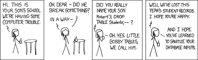
Since an unscrupulous parent might try to smuggle commands into our queries in many different ways, the safest way to deal with this threat is to replace characters like quotes with their escaped equivalents, so that we can safely put whatever the user gives us inside a string. We can do this by using a prepared statement instead of formatting our statements as strings. Here’s what our example program looks like if we do this:
R
library(RSQLite)
connection <- dbConnect(SQLite(), "survey.db")

getName <- function(personID) {
  query <- "SELECT personal || ' ' || family FROM Person WHERE id == ?"
  return(dbGetPreparedQuery(connection, query, data.frame(personID)))
}

print(paste("full name for dyer:", getName('dyer')))

dbDisconnect(connection)
OUTPUT
full name for dyer: William DyerThe key changes are in the query string and the
dbGetQuery call (we use dbGetPreparedQuery instead).
Instead of formatting the query ourselves, we put question marks in the
query template where we want to insert values. When we call
dbGetPreparedQuery, we provide a dataframe that contains as
many values as there are question marks in the query. The library
matches values to question marks in order, and translates any special
characters in the values into their escaped equivalents so that they are
safe to use.
Filling a Table vs. Printing Values
Write an R program that creates a new database in a file called
original.db containing a single table called
Pressure, with a single field called reading,
and inserts 100,000 random numbers between 10.0 and 25.0. How long does
it take this program to run? How long does it take to run a program that
simply writes those random numbers to a file?
Filtering in SQL vs. Filtering in R
Write an R program that creates a new database called
backup.db with the same structure as
original.db and copies all the values greater than 20.0
from original.db to backup.db. Which is
faster: filtering values in the query, or reading everything into memory
and filtering in R?
Database helper functions in R
R’s database interface packages (like RSQLite) all share
a common set of helper functions useful for exploring databases and
reading/writing entire tables at once.
To view all tables in a database, we can use
dbListTables():
R
connection <- dbConnect(SQLite(), "survey.db")
dbListTables(connection)
OUTPUT
"Person" "Site" "Survey" "Visited"To view all column names of a table, use
dbListFields():
R
dbListFields(connection, "Survey")
OUTPUT
"taken" "person" "quant" "reading"To read an entire table as a dataframe, use
dbReadTable():
R
dbReadTable(connection, "Person")
OUTPUT
        id  personal   family
1     dyer   William     Dyer
2       pb     Frank  Pabodie
3     lake  Anderson     Lake
4      roe Valentina  Roerich
5 danforth     Frank Danforth
Finally to write an entire table to a database, you can use
dbWriteTable(). Note that we will always want to use the
row.names = FALSE argument or R will write the row names as
a separate column. In this example we will write R’s built-in
iris dataset as a table in survey.db.
R
dbWriteTable(connection, "iris", iris, row.names = FALSE)
head(dbReadTable(connection, "iris"))
OUTPUT
  Sepal.Length Sepal.Width Petal.Length Petal.Width Species
1          5.1         3.5          1.4         0.2  setosa
2          4.9         3.0          1.4         0.2  setosa
3          4.7         3.2          1.3         0.2  setosa
4          4.6         3.1          1.5         0.2  setosa
5          5.0         3.6          1.4         0.2  setosa
6          5.4         3.9          1.7         0.4  setosa
And as always, remember to close the database connection when done!
R
dbDisconnect(connection)
- Data analysis languages have libraries for accessing databases.
- To connect to a database, a program must use a library specific to that database manager.
- R’s libraries can be used to directly query or read from a database.
- Programs can read query results in batches or all at once.
- Queries should be written using parameter substitution, not string formatting.
- R has multiple helper functions to make working with databases easier.