Plotting and Programming in Python: All in One View

Last updated on 2024-04-15 | Edit this page

Overview

Questions

How can I run Python programs?

Objectives

Launch the JupyterLab server.
Create a new Python script.
Create a Jupyter notebook.
Shutdown the JupyterLab server.
Understand the difference between a Python script and a Jupyter notebook.
Create Markdown cells in a notebook.
Create and run Python cells in a notebook.

To run Python, we are going to use Jupyter Notebooks via JupyterLab for the remainder of this workshop. Jupyter notebooks are common in data science and visualization and serve as a convenient common-denominator experience for running Python code interactively where we can easily view and share the results of our Python code.

There are other ways of editing, managing, and running code. Software developers often use an integrated development environment (IDE) like PyCharm or Visual Studio Code, or text editors like Vim or Emacs, to create and edit their Python programs. After editing and saving your Python programs you can execute those programs within the IDE itself or directly on the command line. In contrast, Jupyter notebooks let us execute and view the results of our Python code immediately within the notebook.

JupyterLab has several other handy features:

You can easily type, edit, and copy and paste blocks of code.
Tab complete allows you to easily access the names of things you are using and learn more about them.
It allows you to annotate your code with links, different sized text, bullets, etc. to make it more accessible to you and your collaborators.
It allows you to display figures next to the code that produces them to tell a complete story of the analysis.

Each notebook contains one or more cells that contain code, text, or images.

Getting Started with JupyterLab

JupyterLab is an application server with a web user interface from Project Jupyter that enables one to work with documents and activities such as Jupyter notebooks, text editors, terminals, and even custom components in a flexible, integrated, and extensible manner. JupyterLab requires a reasonably up-to-date browser (ideally a current version of Chrome, Safari, or Firefox); Internet Explorer versions 9 and below are not supported.

JupyterLab is included as part of the Anaconda Python distribution. If you have not already installed the Anaconda Python distribution, see the setup instructions for installation instructions.

In this lesson we will run JupyterLab locally on our own machines so it will not require an internet connection besides the initial connection to download and install Anaconda and JupyterLab

Start the JupyterLab server on your machine
Use a web browser to open a special localhost URL that connects to your JupyterLab server
The JupyterLab server does the work and the web browser renders the result
Type code into the browser and see the results after your JupyterLab server has finished executing your code

JupyterLab? What about Jupyter notebooks?

JupyterLab is the next stage in the evolution of the Jupyter Notebook. If you have prior experience working with Jupyter notebooks, then you will have a good idea of what to expect from JupyterLab.

Experienced users of Jupyter notebooks interested in a more detailed discussion of the similarities and differences between the JupyterLab and Jupyter notebook user interfaces can find more information in the JupyterLab user interface documentation.

Starting JupyterLab

You can start the JupyterLab server through the command line or through an application called Anaconda Navigator. Anaconda Navigator is included as part of the Anaconda Python distribution.

macOS - Command Line

To start the JupyterLab server you will need to access the command line through the Terminal. There are two ways to open Terminal on Mac.

In your Applications folder, open Utilities and double-click on Terminal
Press Command + spacebar to launch Spotlight. Type Terminal and then double-click the search result or hit Enter

After you have launched Terminal, type the command to launch the JupyterLab server.

BASH

$ jupyter lab

Windows Users - Command Line

To start the JupyterLab server you will need to access the Anaconda Prompt.

Press Windows Logo Key and search for Anaconda Prompt, click the result or press enter.

After you have launched the Anaconda Prompt, type the command:

BASH

$ jupyter lab

Anaconda Navigator

To start a JupyterLab server from Anaconda Navigator you must first start Anaconda Navigator (click for detailed instructions on macOS, Windows, and Linux). You can search for Anaconda Navigator via Spotlight on macOS (Command + spacebar), the Windows search function (Windows Logo Key) or opening a terminal shell and executing the anaconda-navigator executable from the command line.

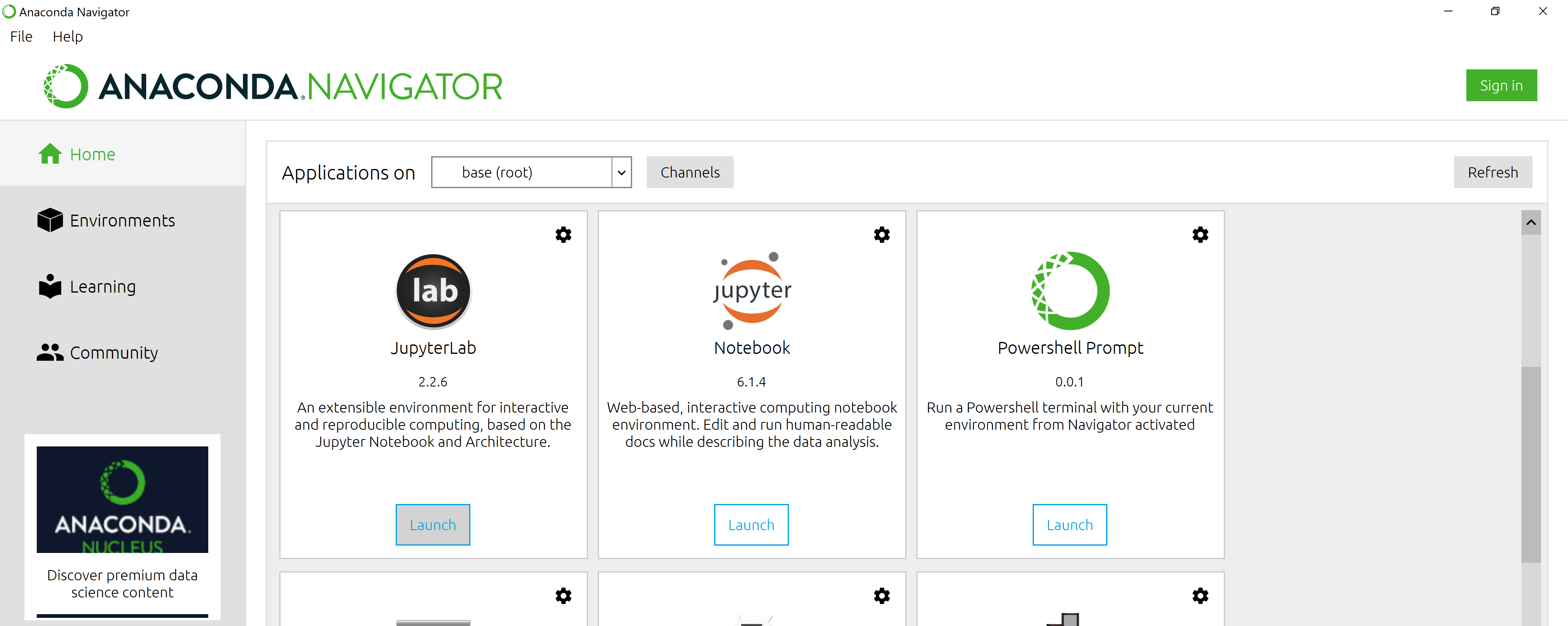
After you have launched Anaconda Navigator, click the Launch button under JupyterLab. You may need to scroll down to find it.

Here is a screenshot of an Anaconda Navigator page similar to the one that should open on either macOS or Windows.

Anaconda Navigator landing page

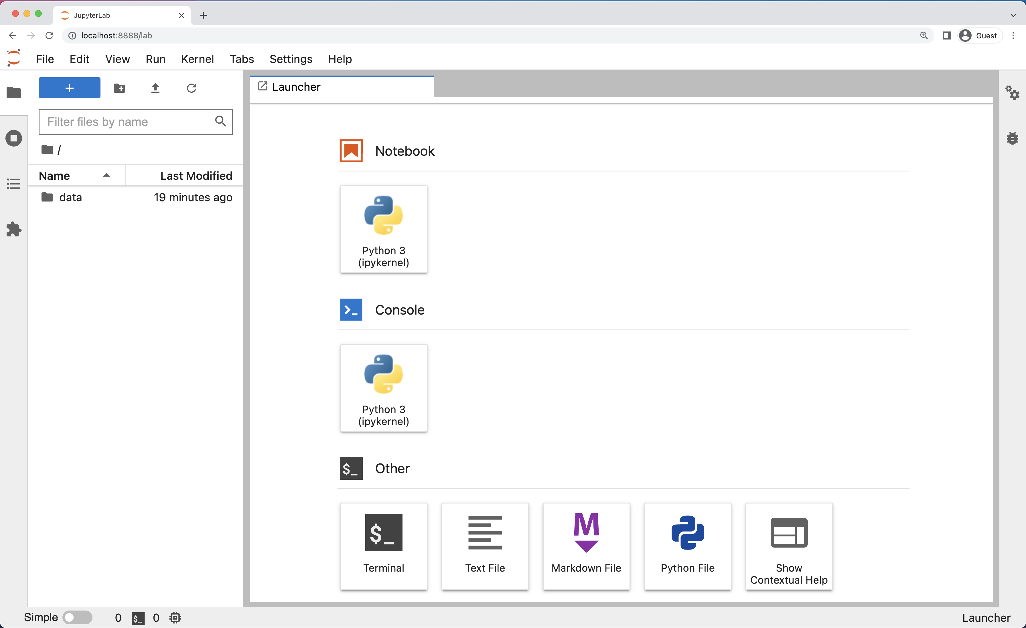
And here is a screenshot of a JupyterLab landing page that should be similar to the one that opens in your default web browser after starting the JupyterLab server on either macOS or Windows.

JupyterLab landing page

The JupyterLab Interface

JupyterLab has many features found in traditional integrated development environments (IDEs) but is focused on providing flexible building blocks for interactive, exploratory computing.

The JupyterLab Interface consists of the Menu Bar, a collapsable Left Side Bar, and the Main Work Area which contains tabs of documents and activities.

The Menu Bar at the top of JupyterLab has the top-level menus that expose various actions available in JupyterLab along with their keyboard shortcuts (where applicable). The following menus are included by default.

File: Actions related to files and directories such as New, Open, Close, Save, etc. The File menu also includes the Shut Down action used to shutdown the JupyterLab server.
Edit: Actions related to editing documents and other activities such as Undo, Cut, Copy, Paste, etc.
View: Actions that alter the appearance of JupyterLab.
Run: Actions for running code in different activities such as notebooks and code consoles (discussed below).
Kernel: Actions for managing kernels. Kernels in Jupyter will be explained in more detail below.
Tabs: A list of the open documents and activities in the main work area.
Settings: Common JupyterLab settings can be configured using this menu. There is also an Advanced Settings Editor option in the dropdown menu that provides more fine-grained control of JupyterLab settings and configuration options.
Help: A list of JupyterLab and kernel help links.

Kernels

The JupyterLab docs define kernels as “separate processes started by the server that runs your code in different programming languages and environments.” When we open a Jupyter Notebook, that starts a kernel - a process - that is going to run the code. In this lesson, we’ll be using the Jupyter ipython kernel which lets us run Python 3 code interactively.

Using other Jupyter kernels for other programming languages would let us write and execute code in other programming languages in the same JupyterLab interface, like R, Java, Julia, Ruby, JavaScript, Fortran, etc.

A screenshot of the default Menu Bar is provided below.

JupyterLab Menu Bar

The left sidebar contains a number of commonly used tabs, such as a file browser (showing the contents of the directory where the JupyterLab server was launched), a list of running kernels and terminals, the command palette, and a list of open tabs in the main work area. A screenshot of the default Left Side Bar is provided below.

JupyterLab Left Side Bar

The left sidebar can be collapsed or expanded by selecting “Show Left Sidebar” in the View menu or by clicking on the active sidebar tab.

Main Work Area

The main work area in JupyterLab enables you to arrange documents (notebooks, text files, etc.) and other activities (terminals, code consoles, etc.) into panels of tabs that can be resized or subdivided. A screenshot of the default Main Work Area is provided below.

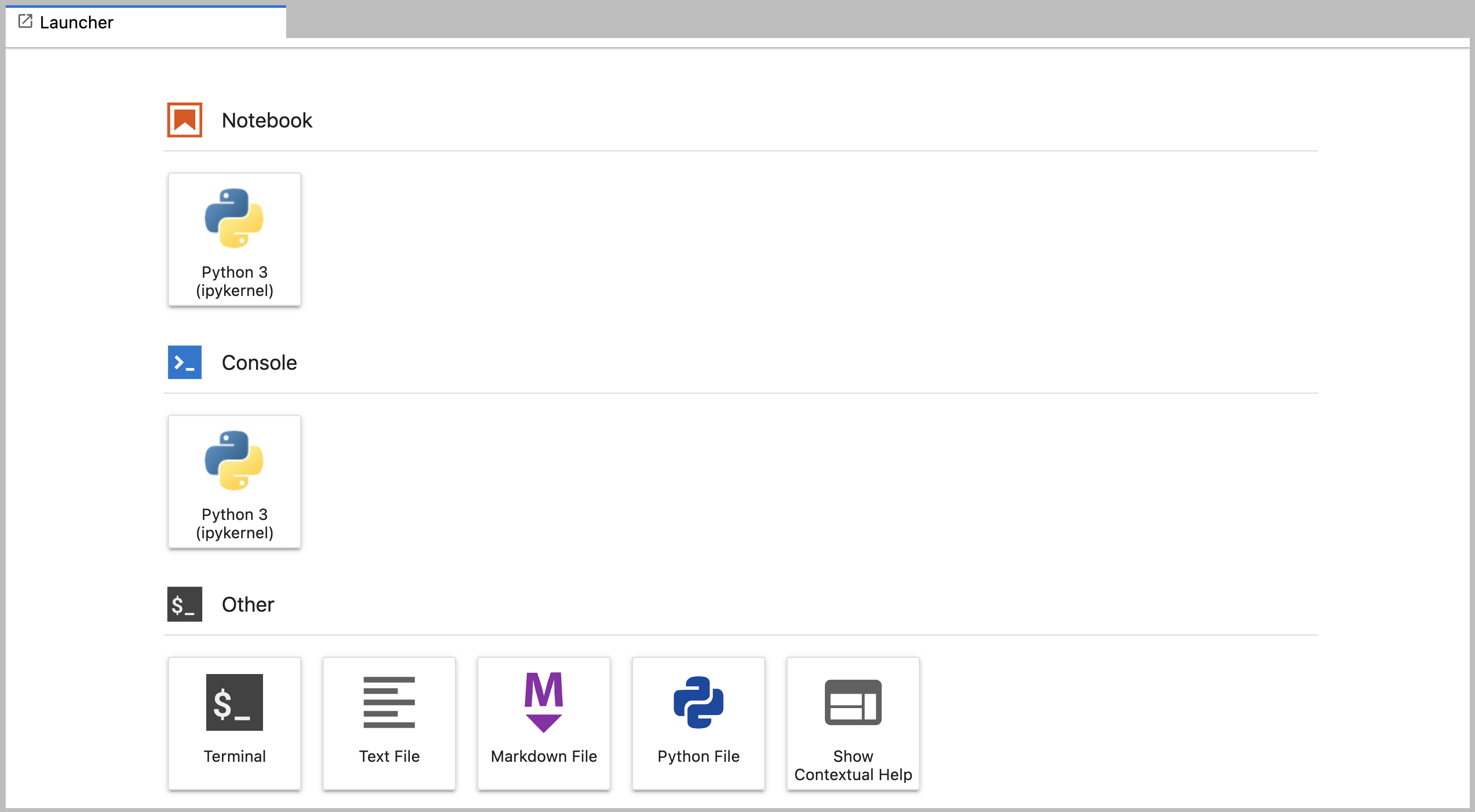
If you do not see the Launcher tab, click the blue plus sign under the “File” and “Edit” menus and it will appear.

JupyterLab Main Work Area

Drag a tab to the center of a tab panel to move the tab to the panel. Subdivide a tab panel by dragging a tab to the left, right, top, or bottom of the panel. The work area has a single current activity. The tab for the current activity is marked with a colored top border (blue by default).

Creating a Python script

To start writing a new Python program click the Text File icon under the Other header in the Launcher tab of the Main Work Area.
- You can also create a new plain text file by selecting the New -> Text File from the File menu in the Menu Bar.
To convert this plain text file to a Python program, select the Save File As action from the File menu in the Menu Bar and give your new text file a name that ends with the .py extension.
- The .py extension lets everyone (including the operating system) know that this text file is a Python program.
- This is convention, not a requirement.

Creating a Jupyter Notebook

To open a new notebook click the Python 3 icon under the Notebook header in the Launcher tab in the main work area. You can also create a new notebook by selecting New -> Notebook from the File menu in the Menu Bar.

Additional notes on Jupyter notebooks.

Notebook files have the extension .ipynb to distinguish them from plain-text Python programs.
Notebooks can be exported as Python scripts that can be run from the command line.

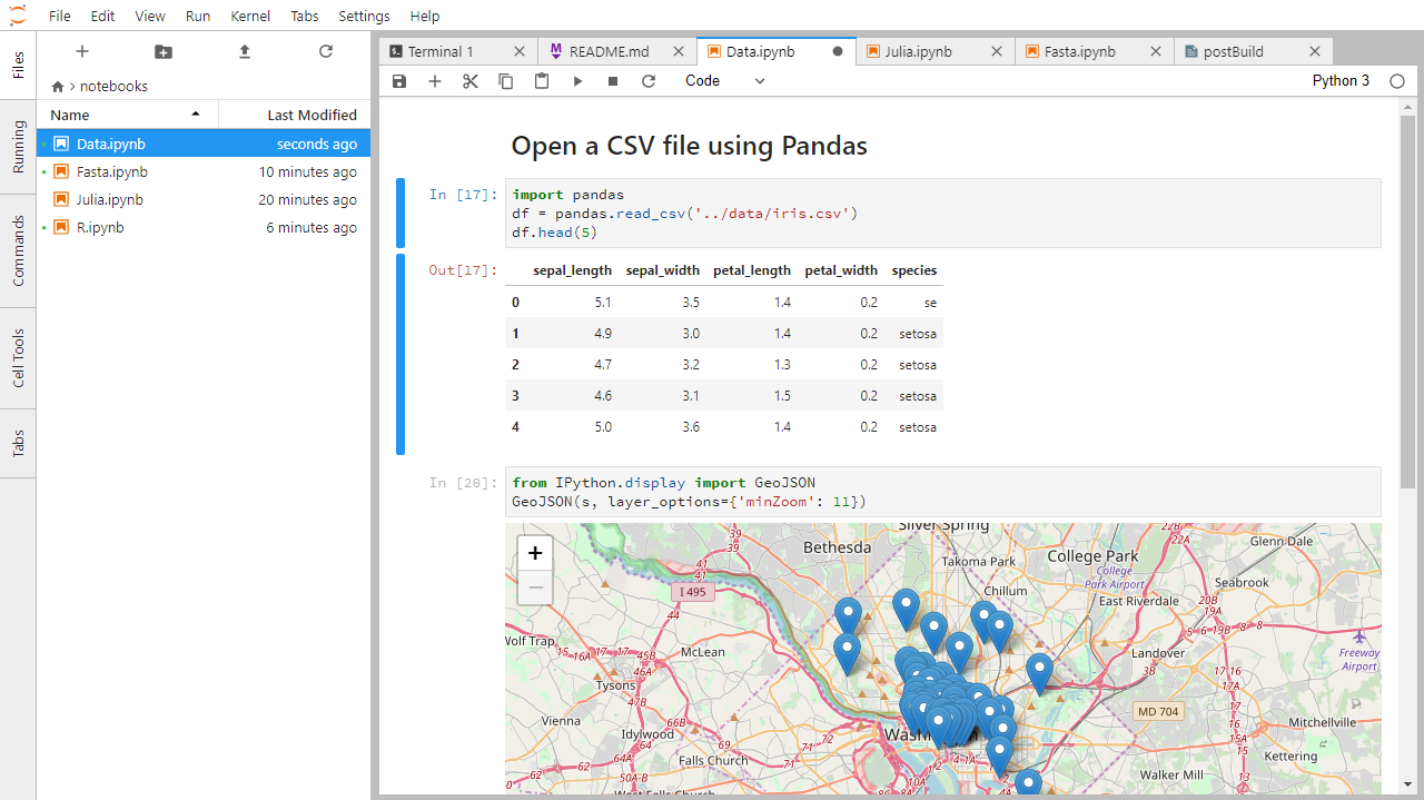
Below is a screenshot of a Jupyter notebook running inside JupyterLab. If you are interested in more details, then see the official notebook documentation.

Example Jupyter Notebook

How It’s Stored

The notebook file is stored in a format called JSON.
Just like a webpage, what’s saved looks different from what you see in your browser.
But this format allows Jupyter to mix source code, text, and images, all in one file.

Arranging Documents into Panels of Tabs

In the JupyterLab Main Work Area you can arrange documents into panels of tabs. Here is an example from the official documentation.

Multi-panel JupyterLab

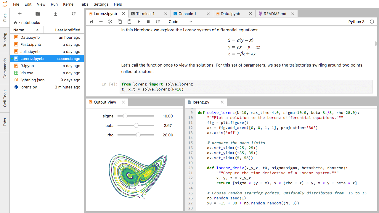
First, create a text file, Python console, and terminal window and arrange them into three panels in the main work area. Next, create a notebook, terminal window, and text file and arrange them into three panels in the main work area. Finally, create your own combination of panels and tabs. What combination of panels and tabs do you think will be most useful for your workflow?

Show me the solution

After creating the necessary tabs, you can drag one of the tabs to the center of a panel to move the tab to the panel; next you can subdivide a tab panel by dragging a tab to the left, right, top, or bottom of the panel.

Code vs. Text

Jupyter mixes code and text in different types of blocks, called cells. We often use the term “code” to mean “the source code of software written in a language such as Python”. A “code cell” in a Notebook is a cell that contains software; a “text cell” is one that contains ordinary prose written for human beings.

The Notebook has Command and Edit modes.

If you press Esc and Return alternately, the outer border of your code cell will change from gray to blue.
These are the Command (gray) and Edit (blue) modes of your notebook.
Command mode allows you to edit notebook-level features, and Edit mode changes the content of cells.
When in Command mode (esc/gray),
- The b key will make a new cell below the currently selected cell.
- The a key will make one above.
- The x key will delete the current cell.
- The z key will undo your last cell operation (which could be a deletion, creation, etc).
All actions can be done using the menus, but there are lots of keyboard shortcuts to speed things up.

Command Vs. Edit

In the Jupyter notebook page are you currently in Command or Edit mode?
Switch between the modes. Use the shortcuts to generate a new cell. Use the shortcuts to delete a cell. Use the shortcuts to undo the last cell operation you performed.

Show me the solution

Command mode has a grey border and Edit mode has a blue border. Use Esc and Return to switch between modes. You need to be in Command mode (Press Esc if your cell is blue). Type b or a. You need to be in Command mode (Press Esc if your cell is blue). Type x. You need to be in Command mode (Press Esc if your cell is blue). Type z.

Use the keyboard and mouse to select and edit cells.

Pressing the Return key turns the border blue and engages Edit mode, which allows you to type within the cell.
Because we want to be able to write many lines of code in a single cell, pressing the Return key when in Edit mode (blue) moves the cursor to the next line in the cell just like in a text editor.
We need some other way to tell the Notebook we want to run what’s in the cell.
Pressing Shift+Return together will execute the contents of the cell.
Notice that the Return and Shift keys on the right of the keyboard are right next to each other.

The Notebook will turn Markdown into pretty-printed documentation.

Notebooks can also render Markdown.
- A simple plain-text format for writing lists, links, and other things that might go into a web page.
- Equivalently, a subset of HTML that looks like what you’d send in an old-fashioned email.
Turn the current cell into a Markdown cell by entering the Command mode (Esc/gray) and press the M key.
In [ ]: will disappear to show it is no longer a code cell and you will be able to write in Markdown.
Turn the current cell into a Code cell by entering the Command mode (Esc/gray) and press the y key.

Markdown does most of what HTML does.

Showing some markdown syntax and its rendered output.
Markdown code	Rendered output

`* Use asterisks * to create * bullet lists.`	Use asterisks to create bullet lists.

`1. Use numbers 1. to create 1. bullet lists.`	Use numbers to create numbered lists.

`* You can use indents * To create sublists * of the same type * Or sublists 1. Of different 1. types`	You can use indents To create sublists of the same type Or sublists Of different types

`# A Level-1 Heading`	A Level-1 Heading

`## A Level-2 Heading (etc.)`	A Level-2 Heading (etc.)

`Line breaks don't matter. But blank lines create new paragraphs.`	Line breaks don’t matter. But blank lines create new paragraphs.

[Links](http://software-carpentry.org) are created with `[...](...)`. Or use [named links][data-carp]. [data-carp]: http://datacarpentry.org	Links are created with `[...](...)`. Or use named links.

Creating Lists in Markdown

Create a nested list in a Markdown cell in a notebook that looks like this:

Get funding.
Do work.

Design experiment.
Collect data.
Analyze.

Write up.
Publish.

Show me the solution

This challenge integrates both the numbered list and bullet list. Note that the bullet list is indented 2 spaces so that it is inline with the items of the numbered list.

1.  Get funding.
2.  Do work.
    *   Design experiment.
    *   Collect data.
    *   Analyze.
3.  Write up.
4.  Publish.

More Math

What is displayed when a Python cell in a notebook that contains several calculations is executed? For example, what happens when this cell is executed?

PYTHON

7 * 3
2 + 1

Show me the solution

Python returns the output of the last calculation.

PYTHON

Change an Existing Cell from Code to Markdown

What happens if you write some Python in a code cell and then you switch it to a Markdown cell? For example, put the following in a code cell:

PYTHON

x = 6 * 7 + 12
print(x)

And then run it with Shift+Return to be sure that it works as a code cell. Now go back to the cell and use Esc then m to switch the cell to Markdown and “run” it with Shift+Return. What happened and how might this be useful?

Show me the solution

The Python code gets treated like Markdown text. The lines appear as if they are part of one contiguous paragraph. This could be useful to temporarily turn on and off cells in notebooks that get used for multiple purposes.

PYTHON

x = 6 * 7 + 12 print(x)

Equations

Standard Markdown (such as we’re using for these notes) won’t render equations, but the Notebook will. Create a new Markdown cell and enter the following:

$\sum_{i=1}^{N} 2^{-i} \approx 1$

(It’s probably easier to copy and paste.) What does it display? What do you think the underscore, _, circumflex, ^, and dollar sign, $, do?

Show me the solution

The notebook shows the equation as it would be rendered from LaTeX equation syntax. The dollar sign, $, is used to tell Markdown that the text in between is a LaTeX equation. If you’re not familiar with LaTeX, underscore, _, is used for subscripts and circumflex, ^, is used for superscripts. A pair of curly braces, { and }, is used to group text together so that the statement i=1 becomes the subscript and N becomes the superscript. Similarly, -i is in curly braces to make the whole statement the superscript for 2. \sum and \approx are LaTeX commands for “sum over” and “approximate” symbols.

Closing JupyterLab

From the Menu Bar select the “File” menu and then choose “Shut Down” at the bottom of the dropdown menu. You will be prompted to confirm that you wish to shutdown the JupyterLab server (don’t forget to save your work!). Click “Shut Down” to shutdown the JupyterLab server.
To restart the JupyterLab server you will need to re-run the following command from a shell.

$ jupyter lab

Closing JupyterLab

Practice closing and restarting the JupyterLab server.

Key Points

Python scripts are plain text files.
Use the Jupyter Notebook for editing and running Python.
The Notebook has Command and Edit modes.
Use the keyboard and mouse to select and edit cells.
The Notebook will turn Markdown into pretty-printed documentation.
Markdown does most of what HTML does.

Content from Variables and Assignment

Last updated on 2023-05-02 | Edit this page

Overview

Questions

How can I store data in programs?

Objectives

Write programs that assign scalar values to variables and perform calculations with those values.
Correctly trace value changes in programs that use scalar assignment.

Use variables to store values.

Variables are names for values.
Variable names
- can only contain letters, digits, and underscore _ (typically used to separate words in long variable names)
- cannot start with a digit
- are case sensitive (age, Age and AGE are three different variables)
The name should also be meaningful so you or another programmer know what it is
Variable names that start with underscores like __alistairs_real_age have a special meaning so we won’t do that until we understand the convention.
In Python the = symbol assigns the value on the right to the name on the left.
The variable is created when a value is assigned to it.
Here, Python assigns an age to a variable age and a name in quotes to a variable first_name.
PYTHON
```
age = 42
first_name = 'Ahmed'
```

Use `print` to display values.

Python has a built-in function called print that prints things as text.
Call the function (i.e., tell Python to run it) by using its name.
Provide values to the function (i.e., the things to print) in parentheses.
To add a string to the printout, wrap the string in single or double quotes.
The values passed to the function are called arguments

PYTHON

print(first_name, 'is', age, 'years old')

OUTPUT

Ahmed is 42 years old

print automatically puts a single space between items to separate them.
And wraps around to a new line at the end.

Variables must be created before they are used.

If a variable doesn’t exist yet, or if the name has been mis-spelled, Python reports an error. (Unlike some languages, which “guess” a default value.)

PYTHON

print(last_name)

ERROR

---------------------------------------------------------------------------
NameError                                 Traceback (most recent call last)
<ipython-input-1-c1fbb4e96102> in <module>()
----> 1 print(last_name)

NameError: name 'last_name' is not defined

The last line of an error message is usually the most informative.
We will look at error messages in detail later.

Variables Persist Between Cells

Be aware that it is the order of execution of cells that is important in a Jupyter notebook, not the order in which they appear. Python will remember all the code that was run previously, including any variables you have defined, irrespective of the order in the notebook. Therefore if you define variables lower down the notebook and then (re)run cells further up, those defined further down will still be present. As an example, create two cells with the following content, in this order:

PYTHON

print(myval)

PYTHON

myval = 1

If you execute this in order, the first cell will give an error. However, if you run the first cell after the second cell it will print out 1. To prevent confusion, it can be helpful to use the Kernel -> Restart & Run All option which clears the interpreter and runs everything from a clean slate going top to bottom.

Variables can be used in calculations.

We can use variables in calculations just as if they were values.
- Remember, we assigned the value 42 to age a few lines ago.

PYTHON

age = age + 3
print('Age in three years:', age)

OUTPUT

Age in three years: 45

Use an index to get a single character from a string.

The characters (individual letters, numbers, and so on) in a string are ordered. For example, the string 'AB' is not the same as 'BA'. Because of this ordering, we can treat the string as a list of characters.
Each position in the string (first, second, etc.) is given a number. This number is called an index or sometimes a subscript.
Indices are numbered from 0.
Use the position’s index in square brackets to get the character at that position.

PYTHON

atom_name = 'helium'
print(atom_name[0])

OUTPUT

Use a slice to get a substring.

A part of a string is called a substring. A substring can be as short as a single character.
An item in a list is called an element. Whenever we treat a string as if it were a list, the string’s elements are its individual characters.
A slice is a part of a string (or, more generally, a part of any list-like thing).
We take a slice with the notation [start:stop], where start is the integer index of the first element we want and stop is the integer index of the element just after the last element we want.
The difference between stop and start is the slice’s length.
Taking a slice does not change the contents of the original string. Instead, taking a slice returns a copy of part of the original string.

PYTHON

atom_name = 'sodium'
print(atom_name[0:3])

OUTPUT

sod

Use the built-in function `len` to find the length of a string.

PYTHON

print(len('helium'))

OUTPUT

Nested functions are evaluated from the inside out, like in mathematics.

Python is case-sensitive.

Python thinks that upper- and lower-case letters are different, so Name and name are different variables.
There are conventions for using upper-case letters at the start of variable names so we will use lower-case letters for now.

Use meaningful variable names.

Python doesn’t care what you call variables as long as they obey the rules (alphanumeric characters and the underscore).

PYTHON

flabadab = 42
ewr_422_yY = 'Ahmed'
print(ewr_422_yY, 'is', flabadab, 'years old')

Use meaningful variable names to help other people understand what the program does.
The most important “other person” is your future self.

Swapping Values

Fill the table showing the values of the variables in this program after each statement is executed.

PYTHON

# Command  # Value of x   # Value of y   # Value of swap #
x = 1.0    #              #              #               #
y = 3.0    #              #              #               #
swap = x   #              #              #               #
x = y      #              #              #               #
y = swap   #              #              #               #

Show me the solution

OUTPUT

# Command  # Value of x   # Value of y   # Value of swap #
x = 1.0    # 1.0          # not defined  # not defined   #
y = 3.0    # 1.0          # 3.0          # not defined   #
swap = x   # 1.0          # 3.0          # 1.0           #
x = y      # 3.0          # 3.0          # 1.0           #
y = swap   # 3.0          # 1.0          # 1.0           #

These three lines exchange the values in x and y using the swap variable for temporary storage. This is a fairly common programming idiom.

Predicting Values

What is the final value of position in the program below? (Try to predict the value without running the program, then check your prediction.)

PYTHON

initial = 'left'
position = initial
initial = 'right'

Show me the solution

PYTHON

print(position)

OUTPUT

left

The initial variable is assigned the value 'left'. In the second line, the position variable also receives the string value 'left'. In third line, the initial variable is given the value 'right', but the position variable retains its string value of 'left'.

Challenge

If you assign a = 123, what happens if you try to get the second digit of a via a[1]?

Show me the solution

Numbers are not strings or sequences and Python will raise an error if you try to perform an index operation on a number. In the next lesson on types and type conversion we will learn more about types and how to convert between different types. If you want the Nth digit of a number you can convert it into a string using the str built-in function and then perform an index operation on that string.

PYTHON

a = 123
print(a[1])

ERROR

TypeError: 'int' object is not subscriptable

PYTHON

a = str(123)
print(a[1])

OUTPUT

Choosing a Name

Which is a better variable name, m, min, or minutes? Why? Hint: think about which code you would rather inherit from someone who is leaving the lab:

ts = m * 60 + s
tot_sec = min * 60 + sec
total_seconds = minutes * 60 + seconds

Show me the solution

minutes is better because min might mean something like “minimum” (and actually is an existing built-in function in Python that we will cover later).

Slicing practice

What does the following program print?

PYTHON

atom_name = 'carbon'
print('atom_name[1:3] is:', atom_name[1:3])

Show me the solution

OUTPUT

atom_name[1:3] is: ar

Slicing concepts

Given the following string:

PYTHON

species_name = "Acacia buxifolia"

What would these expressions return?

species_name[2:8]
species_name[11:] (without a value after the colon)
species_name[:4] (without a value before the colon)
species_name[:] (just a colon)
species_name[11:-3]
species_name[-5:-3]
What happens when you choose a stop value which is out of range? (i.e., try species_name[0:20] or species_name[:103])

Solutions

species_name[2:8] returns the substring 'acia b'
species_name[11:] returns the substring 'folia', from position 11 until the end
species_name[:4] returns the substring 'Acac', from the start up to but not including position 4
species_name[:] returns the entire string 'Acacia buxifolia'
species_name[11:-3] returns the substring 'fo', from the 11th position to the third last position
species_name[-5:-3] also returns the substring 'fo', from the fifth last position to the third last
If a part of the slice is out of range, the operation does not fail. species_name[0:20] gives the same result as species_name[0:], and species_name[:103] gives the same result as species_name[:]

Key Points

Use variables to store values.
Use print to display values.
Variables persist between cells.
Variables must be created before they are used.
Variables can be used in calculations.
Use an index to get a single character from a string.
Use a slice to get a substring.
Use the built-in function len to find the length of a string.
Python is case-sensitive.
Use meaningful variable names.

Content from Data Types and Type Conversion

Last updated on 2023-05-02 | Edit this page

Overview

Questions

What kinds of data do programs store?
How can I convert one type to another?

Objectives

Explain key differences between integers and floating point numbers.
Explain key differences between numbers and character strings.
Use built-in functions to convert between integers, floating point numbers, and strings.

Every value has a type.

Every value in a program has a specific type.
Integer (int): represents positive or negative whole numbers like 3 or -512.
Floating point number (float): represents real numbers like 3.14159 or -2.5.
Character string (usually called “string”, str): text.
- Written in either single quotes or double quotes (as long as they match).
- The quote marks aren’t printed when the string is displayed.

Use the built-in function `type` to find the type of a value.

Use the built-in function type to find out what type a value has.
Works on variables as well.
- But remember: the value has the type — the variable is just a label.

PYTHON

print(type(52))

OUTPUT

<class 'int'>

PYTHON

fitness = 'average'
print(type(fitness))

OUTPUT

<class 'str'>

Types control what operations (or methods) can be performed on a given value.

A value’s type determines what the program can do to it.

PYTHON

print(5 - 3)

OUTPUT

PYTHON

print('hello' - 'h')

ERROR

---------------------------------------------------------------------------
TypeError                                 Traceback (most recent call last)
<ipython-input-2-67f5626a1e07> in <module>()
----> 1 print('hello' - 'h')

TypeError: unsupported operand type(s) for -: 'str' and 'str'

You can use the “+” and “*” operators on strings.

“Adding” character strings concatenates them.

PYTHON

full_name = 'Ahmed' + ' ' + 'Walsh'
print(full_name)

OUTPUT

Ahmed Walsh

Multiplying a character string by an integer N creates a new string that consists of that character string repeated N times.
- Since multiplication is repeated addition.

PYTHON

separator = '=' * 10
print(separator)

OUTPUT

==========

Strings have a length (but numbers don’t).

The built-in function len counts the number of characters in a string.

PYTHON

print(len(full_name))

OUTPUT

But numbers don’t have a length (not even zero).

PYTHON

print(len(52))

ERROR

---------------------------------------------------------------------------
TypeError                                 Traceback (most recent call last)
<ipython-input-3-f769e8e8097d> in <module>()
----> 1 print(len(52))

TypeError: object of type 'int' has no len()

Must convert numbers to strings or vice versa when operating on them.

Cannot add numbers and strings.

PYTHON

print(1 + '2')

ERROR

---------------------------------------------------------------------------
TypeError                                 Traceback (most recent call last)
<ipython-input-4-fe4f54a023c6> in <module>()
----> 1 print(1 + '2')

TypeError: unsupported operand type(s) for +: 'int' and 'str'

Not allowed because it’s ambiguous: should 1 + '2' be 3 or '12'?
Some types can be converted to other types by using the type name as a function.

PYTHON

print(1 + int('2'))
print(str(1) + '2')

OUTPUT

3
12

Can mix integers and floats freely in operations.

Integers and floating-point numbers can be mixed in arithmetic.
- Python 3 automatically converts integers to floats as needed.

PYTHON

print('half is', 1 / 2.0)
print('three squared is', 3.0 ** 2)

OUTPUT

half is 0.5
three squared is 9.0

Variables only change value when something is assigned to them.

If we make one cell in a spreadsheet depend on another, and update the latter, the former updates automatically.
This does not happen in programming languages.

PYTHON

variable_one = 1
variable_two = 5 * variable_one
variable_one = 2
print('first is', variable_one, 'and second is', variable_two)

OUTPUT

first is 2 and second is 5

The computer reads the value of variable_one when doing the multiplication, creates a new value, and assigns it to variable_two.
Afterwards, the value of variable_two is set to the new value and not dependent on variable_one so its value does not automatically change when variable_one changes.

Fractions

What type of value is 3.4? How can you find out?

Show me the solution

It is a floating-point number (often abbreviated “float”). It is possible to find out by using the built-in function type().

PYTHON

print(type(3.4))

OUTPUT

<class 'float'>

Automatic Type Conversion

What type of value is 3.25 + 4?

Show me the solution

It is a float: integers are automatically converted to floats as necessary.

PYTHON

result = 3.25 + 4
print(result, 'is', type(result))

OUTPUT

7.25 is <class 'float'>

Choose a Type

What type of value (integer, floating point number, or character string) would you use to represent each of the following? Try to come up with more than one good answer for each problem. For example, in # 1, when would counting days with a floating point variable make more sense than using an integer?

Number of days since the start of the year.
Time elapsed from the start of the year until now in days.
Serial number of a piece of lab equipment.
A lab specimen’s age
Current population of a city.
Average population of a city over time.

Show me the solution

The answers to the questions are:

Integer, since the number of days would lie between 1 and 365.
Floating point, since fractional days are required
Character string if serial number contains letters and numbers, otherwise integer if the serial number consists only of numerals
This will vary! How do you define a specimen’s age? whole days since collection (integer)? date and time (string)?
Choose floating point to represent population as large aggregates (eg millions), or integer to represent population in units of individuals.
Floating point number, since an average is likely to have a fractional part.

Division Types

In Python 3, the // operator performs integer (whole-number) floor division, the / operator performs floating-point division, and the % (or modulo) operator calculates and returns the remainder from integer division:

PYTHON

print('5 // 3:', 5 // 3)
print('5 / 3:', 5 / 3)
print('5 % 3:', 5 % 3)

OUTPUT

5 // 3: 1
5 / 3: 1.6666666666666667
5 % 3: 2

If num_subjects is the number of subjects taking part in a study, and num_per_survey is the number that can take part in a single survey, write an expression that calculates the number of surveys needed to reach everyone once.

Show me the solution

We want the minimum number of surveys that reaches everyone once, which is the rounded up value of num_subjects/ num_per_survey. This is equivalent to performing a floor division with // and adding 1. Before the division we need to subtract 1 from the number of subjects to deal with the case where num_subjects is evenly divisible by num_per_survey.

PYTHON

num_subjects = 600
num_per_survey = 42
num_surveys = (num_subjects - 1) // num_per_survey + 1

print(num_subjects, 'subjects,', num_per_survey, 'per survey:', num_surveys)

OUTPUT

600 subjects, 42 per survey: 15

Strings to Numbers

Where reasonable, float() will convert a string to a floating point number, and int() will convert a floating point number to an integer:

PYTHON

print("string to float:", float("3.4"))
print("float to int:", int(3.4))

OUTPUT

string to float: 3.4
float to int: 3

If the conversion doesn’t make sense, however, an error message will occur.

PYTHON

print("string to float:", float("Hello world!"))

ERROR

---------------------------------------------------------------------------
ValueError                                Traceback (most recent call last)
<ipython-input-5-df3b790bf0a2> in <module>
----> 1 print("string to float:", float("Hello world!"))

ValueError: could not convert string to float: 'Hello world!'

Given this information, what do you expect the following program to do?

What does it actually do?

Why do you think it does that?

PYTHON

print("fractional string to int:", int("3.4"))

Show me the solution

What do you expect this program to do? It would not be so unreasonable to expect the Python 3 int command to convert the string “3.4” to 3.4 and an additional type conversion to 3. After all, Python 3 performs a lot of other magic - isn’t that part of its charm?

PYTHON

int("3.4")

OUTPUT

---------------------------------------------------------------------------
ValueError                                Traceback (most recent call last)
<ipython-input-2-ec6729dfccdc> in <module>
----> 1 int("3.4")
ValueError: invalid literal for int() with base 10: '3.4'

However, Python 3 throws an error. Why? To be consistent, possibly. If you ask Python to perform two consecutive typecasts, you must convert it explicitly in code.

PYTHON

int(float("3.4"))

OUTPUT

Arithmetic with Different Types

Which of the following will return the floating point number 2.0? Note: there may be more than one right answer.

PYTHON

first = 1.0
second = "1"
third = "1.1"

first + float(second)
float(second) + float(third)
first + int(third)
first + int(float(third))
int(first) + int(float(third))
2.0 * second

Show me the solution

Answer: 1 and 4

Complex Numbers

Python provides complex numbers, which are written as 1.0+2.0j. If val is a complex number, its real and imaginary parts can be accessed using dot notation as val.real and val.imag.

PYTHON

a_complex_number = 6 + 2j
print(a_complex_number.real)
print(a_complex_number.imag)

OUTPUT

6.0
2.0

Why do you think Python uses j instead of i for the imaginary part?
What do you expect 1 + 2j + 3 to produce?
What do you expect 4j to be? What about 4 j or 4 + j?

Show me the solution

Standard mathematics treatments typically use i to denote an imaginary number. However, from media reports it was an early convention established from electrical engineering that now presents a technically expensive area to change. Stack Overflow provides additional explanation and discussion.
(4+2j)
4j and Syntax Error: invalid syntax. In the latter cases, j is considered a variable and the statement depends on if j is defined and if so, its assigned value.

Key Points

Every value has a type.
Use the built-in function type to find the type of a value.
Types control what operations can be done on values.
Strings can be added and multiplied.
Strings have a length (but numbers don’t).
Must convert numbers to strings or vice versa when operating on them.
Can mix integers and floats freely in operations.
Variables only change value when something is assigned to them.

Content from Built-in Functions and Help

Last updated on 2023-05-02 | Edit this page

Overview

Questions

How can I use built-in functions?
How can I find out what they do?
What kind of errors can occur in programs?

Objectives

Explain the purpose of functions.
Correctly call built-in Python functions.
Correctly nest calls to built-in functions.
Use help to display documentation for built-in functions.
Correctly describe situations in which SyntaxError and NameError occur.

Use comments to add documentation to programs.

PYTHON

# This sentence isn't executed by Python.
adjustment = 0.5   # Neither is this - anything after '#' is ignored.

A function may take zero or more arguments.

We have seen some functions already — now let’s take a closer look.
An argument is a value passed into a function.
len takes exactly one.
int, str, and float create a new value from an existing one.
print takes zero or more.
print with no arguments prints a blank line.
- Must always use parentheses, even if they’re empty, so that Python knows a function is being called.

PYTHON

print('before')
print()
print('after')

OUTPUT

before

after

Every function returns something.

Every function call produces some result.
If the function doesn’t have a useful result to return, it usually returns the special value None. None is a Python object that stands in anytime there is no value.

PYTHON

result = print('example')
print('result of print is', result)

OUTPUT

example
result of print is None

Commonly-used built-in functions include `max`, `min`, and `round`.

Use max to find the largest value of one or more values.
Use min to find the smallest.
Both work on character strings as well as numbers.
- “Larger” and “smaller” use (0-9, A-Z, a-z) to compare letters.

PYTHON

print(max(1, 2, 3))
print(min('a', 'A', '0'))

OUTPUT

3
0

Functions may only work for certain (combinations of) arguments.

max and min must be given at least one argument.
- “Largest of the empty set” is a meaningless question.
And they must be given things that can meaningfully be compared.

PYTHON

print(max(1, 'a'))

ERROR

TypeError                                 Traceback (most recent call last)
<ipython-input-52-3f049acf3762> in <module>
----> 1 print(max(1, 'a'))

TypeError: '>' not supported between instances of 'str' and 'int'

Functions may have default values for some arguments.

round will round off a floating-point number.
By default, rounds to zero decimal places.

PYTHON

round(3.712)

OUTPUT

We can specify the number of decimal places we want.

PYTHON

round(3.712, 1)

OUTPUT

3.7

Functions attached to objects are called methods

Functions take another form that will be common in the pandas episodes.
Methods have parentheses like functions, but come after the variable.
Some methods are used for internal Python operations, and are marked with double underlines.

PYTHON

my_string = 'Hello world!'  # creation of a string object 

print(len(my_string))       # the len function takes a string as an argument and returns the length of the string

print(my_string.swapcase()) # calling the swapcase method on the my_string object

print(my_string.__len__())  # calling the internal __len__ method on the my_string object, used by len(my_string)

OUTPUT

12
hELLO WORLD!
12

You might even see them chained together. They operate left to right.

PYTHON

print(my_string.isupper())          # Not all the letters are uppercase
print(my_string.upper())            # This capitalizes all the letters

print(my_string.upper().isupper())  # Now all the letters are uppercase

OUTPUT

False
HELLO WORLD
True

Use the built-in function `help` to get help for a function.

Every built-in function has online documentation.

PYTHON

help(round)

OUTPUT

Help on built-in function round in module builtins:

round(number, ndigits=None)
    Round a number to a given precision in decimal digits.

    The return value is an integer if ndigits is omitted or None.  Otherwise
    the return value has the same type as the number.  ndigits may be negative.

The Jupyter Notebook has two ways to get help.

Option 1: Place the cursor near where the function is invoked in a cell (i.e., the function name or its parameters),
- Hold down Shift, and press Tab.
- Do this several times to expand the information returned.
Option 2: Type the function name in a cell with a question mark after it. Then run the cell.

Python reports a syntax error when it can’t understand the source of a program.

Won’t even try to run the program if it can’t be parsed.

PYTHON

# Forgot to close the quote marks around the string.
name = 'Feng

ERROR

  File "<ipython-input-56-f42768451d55>", line 2
    name = 'Feng
                ^
SyntaxError: EOL while scanning string literal

PYTHON

# An extra '=' in the assignment.
age = = 52

ERROR

  File "<ipython-input-57-ccc3df3cf902>", line 2
    age = = 52
          ^
SyntaxError: invalid syntax

Look more closely at the error message:

PYTHON

print("hello world"

ERROR

  File "<ipython-input-6-d1cc229bf815>", line 1
    print ("hello world"
                        ^
SyntaxError: unexpected EOF while parsing

The message indicates a problem on first line of the input (“line 1”).
- In this case the “ipython-input” section of the file name tells us that we are working with input into IPython, the Python interpreter used by the Jupyter Notebook.
The -6- part of the filename indicates that the error occurred in cell 6 of our Notebook.
Next is the problematic line of code, indicating the problem with a ^ pointer.

Python reports a runtime error when something goes wrong while a program is executing.

PYTHON

age = 53
remaining = 100 - aege # mis-spelled 'age'

ERROR

NameError                                 Traceback (most recent call last)
<ipython-input-59-1214fb6c55fc> in <module>
      1 age = 53
----> 2 remaining = 100 - aege # mis-spelled 'age'

NameError: name 'aege' is not defined

Fix syntax errors by reading the source and runtime errors by tracing execution.

What Happens When

Explain in simple terms the order of operations in the following program: when does the addition happen, when does the subtraction happen, when is each function called, etc.
What is the final value of radiance?

PYTHON

radiance = 1.0
radiance = max(2.1, 2.0 + min(radiance, 1.1 * radiance - 0.5))

Show me the solution

Order of operations:
1.1 * radiance = 1.1
1.1 - 0.5 = 0.6
min(radiance, 0.6) = 0.6
2.0 + 0.6 = 2.6
max(2.1, 2.6) = 2.6
At the end, radiance = 2.6

Spot the Difference

Predict what each of the print statements in the program below will print.
Does max(len(rich), poor) run or produce an error message? If it runs, does its result make any sense?

PYTHON

easy_string = "abc"
print(max(easy_string))
rich = "gold"
poor = "tin"
print(max(rich, poor))
print(max(len(rich), len(poor)))

Show me the solution

PYTHON

print(max(easy_string))

OUTPUT

PYTHON

print(max(rich, poor))

OUTPUT

tin

PYTHON

print(max(len(rich), len(poor)))

OUTPUT

max(len(rich), poor) throws a TypeError. This turns into max(4, 'tin') and as we discussed earlier a string and integer cannot meaningfully be compared.

ERROR

TypeError                                 Traceback (most recent call last)
<ipython-input-65-bc82ad05177a> in <module>
----> 1 max(len(rich), poor)

TypeError: '>' not supported between instances of 'str' and 'int'

Why Not?

Why is it that max and min do not return None when they are called with no arguments?

Show me the solution

max and min return TypeErrors in this case because the correct number of parameters was not supplied. If it just returned None, the error would be much harder to trace as it would likely be stored into a variable and used later in the program, only to likely throw a runtime error.

Last Character of a String

If Python starts counting from zero, and len returns the number of characters in a string, what index expression will get the last character in the string name? (Note: we will see a simpler way to do this in a later episode.)

Show me the solution

name[len(name) - 1]

Explore the Python docs!

The official Python documentation is arguably the most complete source of information about the language. It is available in different languages and contains a lot of useful resources. The Built-in Functions page contains a catalogue of all of these functions, including the ones that we’ve covered in this lesson. Some of these are more advanced and unnecessary at the moment, but others are very simple and useful.

Key Points

Use comments to add documentation to programs.
A function may take zero or more arguments.
Commonly-used built-in functions include max, min, and round.
Functions may only work for certain (combinations of) arguments.
Functions may have default values for some arguments.
Use the built-in function help to get help for a function.
The Jupyter Notebook has two ways to get help.
Every function returns something.
Python reports a syntax error when it can’t understand the source of a program.
Python reports a runtime error when something goes wrong while a program is executing.
Fix syntax errors by reading the source code, and runtime errors by tracing the program’s execution.

Content from Morning Coffee

Last updated on 2023-05-02 | Edit this page

Reflection exercise

Over coffee, reflect on and discuss the following:

What are the different kinds of errors Python will report?
Did the code always produce the results you expected? If not, why?
Is there something we can do to prevent errors when we write code?

Content from Libraries

Last updated on 2023-05-02 | Edit this page

Overview

Questions

How can I use software that other people have written?
How can I find out what that software does?

Objectives

Explain what software libraries are and why programmers create and use them.
Write programs that import and use modules from Python’s standard library.
Find and read documentation for the standard library interactively (in the interpreter) and online.

Most of the power of a programming language is in its libraries.

A library is a collection of files (called modules) that contains functions for use by other programs.
- May also contain data values (e.g., numerical constants) and other things.
- Library’s contents are supposed to be related, but there’s no way to enforce that.
The Python standard library is an extensive suite of modules that comes with Python itself.
Many additional libraries are available from PyPI (the Python Package Index).
We will see later how to write new libraries.

Libraries and modules

A library is a collection of modules, but the terms are often used interchangeably, especially since many libraries only consist of a single module, so don’t worry if you mix them.

A program must import a library module before using it.

Use import to load a library module into a program’s memory.
Then refer to things from the module as module_name.thing_name.
- Python uses . to mean “part of”.
Using math, one of the modules in the standard library:

PYTHON

import math

print('pi is', math.pi)
print('cos(pi) is', math.cos(math.pi))

OUTPUT

pi is 3.141592653589793
cos(pi) is -1.0

Have to refer to each item with the module’s name.
- math.cos(pi) won’t work: the reference to pi doesn’t somehow “inherit” the function’s reference to math.

Use `help` to learn about the contents of a library module.

Works just like help for a function.

PYTHON

help(math)

OUTPUT

Help on module math:

NAME
    math

MODULE REFERENCE
    http://docs.python.org/3/library/math

    The following documentation is automatically generated from the Python
    source files.  It may be incomplete, incorrect or include features that
    are considered implementation detail and may vary between Python
    implementations.  When in doubt, consult the module reference at the
    location listed above.

DESCRIPTION
    This module is always available.  It provides access to the
    mathematical functions defined by the C standard.

FUNCTIONS
    acos(x, /)
        Return the arc cosine (measured in radians) of x.
⋮ ⋮ ⋮

Import specific items from a library module to shorten programs.

Use from ... import ... to load only specific items from a library module.
Then refer to them directly without library name as prefix.

PYTHON

from math import cos, pi

print('cos(pi) is', cos(pi))

OUTPUT

cos(pi) is -1.0

Create an alias for a library module when importing it to shorten programs.

Use import ... as ... to give a library a short alias while importing it.
Then refer to items in the library using that shortened name.

PYTHON

import math as m

print('cos(pi) is', m.cos(m.pi))

OUTPUT

cos(pi) is -1.0

Commonly used for libraries that are frequently used or have long names.
- E.g., the matplotlib plotting library is often aliased as mpl.
But can make programs harder to understand, since readers must learn your program’s aliases.

Exploring the Math Module

What function from the math module can you use to calculate a square root without using sqrt?
Since the library contains this function, why does sqrt exist?

Show me the solution

Using help(math) we see that we’ve got pow(x,y) in addition to sqrt(x), so we could use pow(x, 0.5) to find a square root.
The sqrt(x) function is arguably more readable than pow(x, 0.5) when implementing equations. Readability is a cornerstone of good programming, so it makes sense to provide a special function for this specific common case.

Also, the design of Python’s math library has its origin in the C standard, which includes both sqrt(x) and pow(x,y), so a little bit of the history of programming is showing in Python’s function names.

Locating the Right Module

You want to select a random character from a string:

PYTHON

bases = 'ACTTGCTTGAC'

Which standard library module could help you?
Which function would you select from that module? Are there alternatives?
Try to write a program that uses the function.

Show me the solution

The random module seems like it could help.

The string has 11 characters, each having a positional index from 0 to 10. You could use the random.randrange or random.randint functions to get a random integer between 0 and 10, and then select the bases character at that index:

PYTHON

from random import randrange

random_index = randrange(len(bases))
print(bases[random_index])

or more compactly:

PYTHON

from random import randrange

print(bases[randrange(len(bases))])

Perhaps you found the random.sample function? It allows for slightly less typing but might be a bit harder to understand just by reading:

PYTHON

from random import sample

print(sample(bases, 1)[0])

Note that this function returns a list of values. We will learn about lists in episode 11.

The simplest and shortest solution is the random.choice function that does exactly what we want:

PYTHON

from random import choice

print(choice(bases))

Jigsaw Puzzle (Parson’s Problem) Programming Example

Rearrange the following statements so that a random DNA base is printed and its index in the string. Not all statements may be needed. Feel free to use/add intermediate variables.

PYTHON

bases="ACTTGCTTGAC"
import math
import random
___ = random.randrange(n_bases)
___ = len(bases)
print("random base ", bases[___], "base index", ___)

Show me the solution

PYTHON

import math 
import random
bases = "ACTTGCTTGAC" 
n_bases = len(bases)
idx = random.randrange(n_bases)
print("random base", bases[idx], "base index", idx)

When Is Help Available?

When a colleague of yours types help(math), Python reports an error:

ERROR

NameError: name 'math' is not defined

What has your colleague forgotten to do?

Show me the solution

Importing the math module (import math)

Importing With Aliases

Fill in the blanks so that the program below prints 90.0.
Rewrite the program so that it uses import without as.
Which form do you find easier to read?

PYTHON

import math as m
angle = ____.degrees(____.pi / 2)
print(____)

Show me the solution

PYTHON

import math as m
angle = m.degrees(m.pi / 2)
print(angle)

can be written as

PYTHON

import math
angle = math.degrees(math.pi / 2)
print(angle)

Since you just wrote the code and are familiar with it, you might actually find the first version easier to read. But when trying to read a huge piece of code written by someone else, or when getting back to your own huge piece of code after several months, non-abbreviated names are often easier, except where there are clear abbreviation conventions.

There Are Many Ways To Import Libraries!

Match the following print statements with the appropriate library calls.

Print commands:

print("sin(pi/2) =", sin(pi/2))
print("sin(pi/2) =", m.sin(m.pi/2))
print("sin(pi/2) =", math.sin(math.pi/2))

Library calls:

from math import sin, pi
import math
import math as m
from math import *

Show me the solution

Library calls 1 and 4. In order to directly refer to sin and pi without the library name as prefix, you need to use the from ... import ... statement. Whereas library call 1 specifically imports the two functions sin and pi, library call 4 imports all functions in the math module.
Library call 3. Here sin and pi are referred to with a shortened library name m instead of math. Library call 3 does exactly that using the import ... as ... syntax - it creates an alias for math in the form of the shortened name m.
Library call 2. Here sin and pi are referred to with the regular library name math, so the regular import ... call suffices.

Note: although library call 4 works, importing all names from a module using a wildcard import is not recommended as it makes it unclear which names from the module are used in the code. In general it is best to make your imports as specific as possible and to only import what your code uses. In library call 1, the import statement explicitly tells us that the sin function is imported from the math module, but library call 4 does not convey this information.

Importing Specific Items

Fill in the blanks so that the program below prints 90.0.
Do you find this version easier to read than preceding ones?
Why wouldn’t programmers always use this form of import?

PYTHON

____ math import ____, ____
angle = degrees(pi / 2)
print(angle)

Show me the solution

PYTHON

from math import degrees, pi
angle = degrees(pi / 2)
print(angle)

Most likely you find this version easier to read since it’s less dense. The main reason not to use this form of import is to avoid name clashes. For instance, you wouldn’t import degrees this way if you also wanted to use the name degrees for a variable or function of your own. Or if you were to also import a function named degrees from another library.

Reading Error Messages

Read the code below and try to identify what the errors are without running it.
Run the code, and read the error message. What type of error is it?

PYTHON

from math import log
log(0)

Show me the solution

OUTPUT

---------------------------------------------------------------------------
ValueError                                Traceback (most recent call last)
<ipython-input-1-d72e1d780bab> in <module>
      1 from math import log
----> 2 log(0)

ValueError: math domain error

The logarithm of x is only defined for x > 0, so 0 is outside the domain of the function.
You get an error of type ValueError, indicating that the function received an inappropriate argument value. The additional message “math domain error” makes it clearer what the problem is.

Key Points

Most of the power of a programming language is in its libraries.
A program must import a library module in order to use it.
Use help to learn about the contents of a library module.
Import specific items from a library to shorten programs.
Create an alias for a library when importing it to shorten programs.

Content from Reading Tabular Data into DataFrames

Last updated on 2023-05-02 | Edit this page

Overview

Questions

How can I read tabular data?

Objectives

Import the Pandas library.
Use Pandas to load a simple CSV data set.
Get some basic information about a Pandas DataFrame.

Use the Pandas library to do statistics on tabular data.

Pandas is a widely-used Python library for statistics, particularly on tabular data.
Borrows many features from R’s dataframes.
- A 2-dimensional table whose columns have names and potentially have different data types.
Load Pandas with import pandas as pd. The alias pd is commonly used to refer to the Pandas library in code.
Read a Comma Separated Values (CSV) data file with pd.read_csv.
- Argument is the name of the file to be read.
- Returns a dataframe that you can assign to a variable

PYTHON

import pandas as pd

data_oceania = pd.read_csv('data/gapminder_gdp_oceania.csv')
print(data_oceania)

OUTPUT

       country  gdpPercap_1952  gdpPercap_1957  gdpPercap_1962  \
0    Australia     10039.59564     10949.64959     12217.22686
1  New Zealand     10556.57566     12247.39532     13175.67800

   gdpPercap_1967  gdpPercap_1972  gdpPercap_1977  gdpPercap_1982  \
0     14526.12465     16788.62948     18334.19751     19477.00928
1     14463.91893     16046.03728     16233.71770     17632.41040

   gdpPercap_1987  gdpPercap_1992  gdpPercap_1997  gdpPercap_2002  \
0     21888.88903     23424.76683     26997.93657     30687.75473
1     19007.19129     18363.32494     21050.41377     23189.80135

   gdpPercap_2007
0     34435.36744
1     25185.00911

The columns in a dataframe are the observed variables, and the rows are the observations.
Pandas uses backslash \ to show wrapped lines when output is too wide to fit the screen.
Using descriptive dataframe names helps us distinguish between multiple dataframes so we won’t accidentally overwrite a dataframe or read from the wrong one.

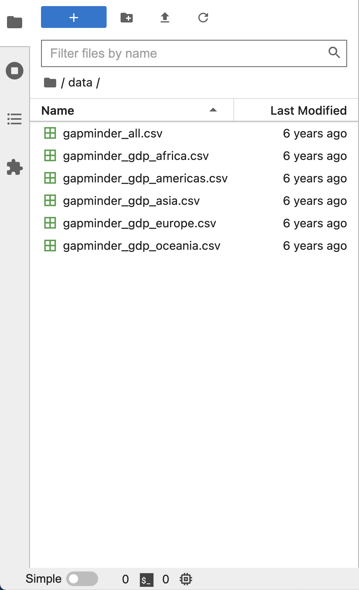
File Not Found

Our lessons store their data files in a data sub-directory, which is why the path to the file is data/gapminder_gdp_oceania.csv. If you forget to include data/, or if you include it but your copy of the file is somewhere else, you will get a runtime error that ends with a line like this:

ERROR

FileNotFoundError: [Errno 2] No such file or directory: 'data/gapminder_gdp_oceania.csv'

Use `index_col` to specify that a column’s values should be used as row headings.

Row headings are numbers (0 and 1 in this case).
Really want to index by country.
Pass the name of the column to read_csv as its index_col parameter to do this.
Naming the dataframe data_oceania_country tells us which region the data includes (oceania) and how it is indexed (country).

PYTHON

data_oceania_country = pd.read_csv('data/gapminder_gdp_oceania.csv', index_col='country')
print(data_oceania_country)

OUTPUT

             gdpPercap_1952  gdpPercap_1957  gdpPercap_1962  gdpPercap_1967  \
country
Australia       10039.59564     10949.64959     12217.22686     14526.12465
New Zealand     10556.57566     12247.39532     13175.67800     14463.91893

             gdpPercap_1972  gdpPercap_1977  gdpPercap_1982  gdpPercap_1987  \
country
Australia       16788.62948     18334.19751     19477.00928     21888.88903
New Zealand     16046.03728     16233.71770     17632.41040     19007.19129

             gdpPercap_1992  gdpPercap_1997  gdpPercap_2002  gdpPercap_2007
country
Australia       23424.76683     26997.93657     30687.75473     34435.36744
New Zealand     18363.32494     21050.41377     23189.80135     25185.00911

Use the `DataFrame.info()` method to find out more about a dataframe.

PYTHON

data_oceania_country.info()

OUTPUT

<class 'pandas.core.frame.DataFrame'>
Index: 2 entries, Australia to New Zealand
Data columns (total 12 columns):
gdpPercap_1952    2 non-null float64
gdpPercap_1957    2 non-null float64
gdpPercap_1962    2 non-null float64
gdpPercap_1967    2 non-null float64
gdpPercap_1972    2 non-null float64
gdpPercap_1977    2 non-null float64
gdpPercap_1982    2 non-null float64
gdpPercap_1987    2 non-null float64
gdpPercap_1992    2 non-null float64
gdpPercap_1997    2 non-null float64
gdpPercap_2002    2 non-null float64
gdpPercap_2007    2 non-null float64
dtypes: float64(12)
memory usage: 208.0+ bytes

This is a DataFrame
Two rows named 'Australia' and 'New Zealand'
Twelve columns, each of which has two actual 64-bit floating point values.
- We will talk later about null values, which are used to represent missing observations.
Uses 208 bytes of memory.

The `DataFrame.columns` variable stores information about the dataframe’s columns.

Note that this is data, not a method. (It doesn’t have parentheses.)
- Like math.pi.
- So do not use () to try to call it.
Called a member variable, or just member.

PYTHON

print(data_oceania_country.columns)

OUTPUT

Index(['gdpPercap_1952', 'gdpPercap_1957', 'gdpPercap_1962', 'gdpPercap_1967',
       'gdpPercap_1972', 'gdpPercap_1977', 'gdpPercap_1982', 'gdpPercap_1987',
       'gdpPercap_1992', 'gdpPercap_1997', 'gdpPercap_2002', 'gdpPercap_2007'],
      dtype='object')

Use `DataFrame.T` to transpose a dataframe.

Sometimes want to treat columns as rows and vice versa.
Transpose (written .T) doesn’t copy the data, just changes the program’s view of it.
Like columns, it is a member variable.

PYTHON

print(data_oceania_country.T)

OUTPUT

country           Australia  New Zealand
gdpPercap_1952  10039.59564  10556.57566
gdpPercap_1957  10949.64959  12247.39532
gdpPercap_1962  12217.22686  13175.67800
gdpPercap_1967  14526.12465  14463.91893
gdpPercap_1972  16788.62948  16046.03728
gdpPercap_1977  18334.19751  16233.71770
gdpPercap_1982  19477.00928  17632.41040
gdpPercap_1987  21888.88903  19007.19129
gdpPercap_1992  23424.76683  18363.32494
gdpPercap_1997  26997.93657  21050.41377
gdpPercap_2002  30687.75473  23189.80135
gdpPercap_2007  34435.36744  25185.00911

Use `DataFrame.describe()` to get summary statistics about data.

DataFrame.describe() gets the summary statistics of only the columns that have numerical data. All other columns are ignored, unless you use the argument include='all'.

PYTHON

print(data_oceania_country.describe())

OUTPUT

       gdpPercap_1952  gdpPercap_1957  gdpPercap_1962  gdpPercap_1967  \
count        2.000000        2.000000        2.000000        2.000000
mean     10298.085650    11598.522455    12696.452430    14495.021790
std        365.560078      917.644806      677.727301       43.986086
min      10039.595640    10949.649590    12217.226860    14463.918930
25%      10168.840645    11274.086022    12456.839645    14479.470360
50%      10298.085650    11598.522455    12696.452430    14495.021790
75%      10427.330655    11922.958888    12936.065215    14510.573220
max      10556.575660    12247.395320    13175.678000    14526.124650

       gdpPercap_1972  gdpPercap_1977  gdpPercap_1982  gdpPercap_1987  \
count         2.00000        2.000000        2.000000        2.000000
mean      16417.33338    17283.957605    18554.709840    20448.040160
std         525.09198     1485.263517     1304.328377     2037.668013
min       16046.03728    16233.717700    17632.410400    19007.191290
25%       16231.68533    16758.837652    18093.560120    19727.615725
50%       16417.33338    17283.957605    18554.709840    20448.040160
75%       16602.98143    17809.077557    19015.859560    21168.464595
max       16788.62948    18334.197510    19477.009280    21888.889030

       gdpPercap_1992  gdpPercap_1997  gdpPercap_2002  gdpPercap_2007
count        2.000000        2.000000        2.000000        2.000000
mean     20894.045885    24024.175170    26938.778040    29810.188275
std       3578.979883     4205.533703     5301.853680     6540.991104
min      18363.324940    21050.413770    23189.801350    25185.009110
25%      19628.685413    22537.294470    25064.289695    27497.598692
50%      20894.045885    24024.175170    26938.778040    29810.188275
75%      22159.406358    25511.055870    28813.266385    32122.777857
max      23424.766830    26997.936570    30687.754730    34435.367440

Not particularly useful with just two records, but very helpful when there are thousands.

Reading Other Data

Read the data in gapminder_gdp_americas.csv (which should be in the same directory as gapminder_gdp_oceania.csv) into a variable called data_americas and display its summary statistics.

Show me the solution

To read in a CSV, we use pd.read_csv and pass the filename 'data/gapminder_gdp_americas.csv' to it. We also once again pass the column name 'country' to the parameter index_col in order to index by country. The summary statistics can be displayed with the DataFrame.describe() method.

PYTHON

data_americas = pd.read_csv('data/gapminder_gdp_americas.csv', index_col='country')
data_americas.describe()

Inspecting Data

After reading the data for the Americas, use help(data_americas.head) and help(data_americas.tail) to find out what DataFrame.head and DataFrame.tail do.

What method call will display the first three rows of this data?
What method call will display the last three columns of this data? (Hint: you may need to change your view of the data.)

Show me the solution

We can check out the first five rows of data_americas by executing data_americas.head() which lets us view the beginning of the DataFrame. We can specify the number of rows we wish to see by specifying the parameter n in our call to data_americas.head(). To view the first three rows, execute:

PYTHON

data_americas.head(n=3)

OUTPUT

          continent  gdpPercap_1952  gdpPercap_1957  gdpPercap_1962  \
country
Argentina  Americas     5911.315053     6856.856212     7133.166023
Bolivia    Americas     2677.326347     2127.686326     2180.972546
Brazil     Americas     2108.944355     2487.365989     3336.585802

          gdpPercap_1967  gdpPercap_1972  gdpPercap_1977  gdpPercap_1982  \
country
Argentina     8052.953021     9443.038526    10079.026740     8997.897412
Bolivia       2586.886053     2980.331339     3548.097832     3156.510452
Brazil        3429.864357     4985.711467     6660.118654     7030.835878

           gdpPercap_1987  gdpPercap_1992  gdpPercap_1997  gdpPercap_2002  \
country
Argentina     9139.671389     9308.418710    10967.281950     8797.640716
Bolivia       2753.691490     2961.699694     3326.143191     3413.262690
Brazil        7807.095818     6950.283021     7957.980824     8131.212843

           gdpPercap_2007
country
Argentina    12779.379640
Bolivia       3822.137084
Brazil        9065.800825

To check out the last three rows of data_americas, we would use the command, americas.tail(n=3), analogous to head() used above. However, here we want to look at the last three columns so we need to change our view and then use tail(). To do so, we create a new DataFrame in which rows and columns are switched:

PYTHON

americas_flipped = data_americas.T

We can then view the last three columns of americas by viewing the last three rows of americas_flipped:

PYTHON

americas_flipped.tail(n=3)

OUTPUT

country        Argentina  Bolivia   Brazil   Canada    Chile Colombia  \
gdpPercap_1997   10967.3  3326.14  7957.98  28954.9  10118.1  6117.36
gdpPercap_2002   8797.64  3413.26  8131.21    33329  10778.8  5755.26
gdpPercap_2007   12779.4  3822.14   9065.8  36319.2  13171.6  7006.58

country        Costa Rica     Cuba Dominican Republic  Ecuador    ...     \
gdpPercap_1997    6677.05  5431.99             3614.1  7429.46    ...
gdpPercap_2002    7723.45  6340.65            4563.81  5773.04    ...
gdpPercap_2007    9645.06   8948.1            6025.37  6873.26    ...

country          Mexico Nicaragua   Panama Paraguay     Peru Puerto Rico  \
gdpPercap_1997   9767.3   2253.02  7113.69   4247.4  5838.35     16999.4
gdpPercap_2002  10742.4   2474.55  7356.03  3783.67  5909.02     18855.6
gdpPercap_2007  11977.6   2749.32  9809.19  4172.84  7408.91     19328.7

country        Trinidad and Tobago United States  Uruguay Venezuela
gdpPercap_1997             8792.57       35767.4  9230.24   10165.5
gdpPercap_2002             11460.6       39097.1     7727   8605.05
gdpPercap_2007             18008.5       42951.7  10611.5   11415.8

This shows the data that we want, but we may prefer to display three columns instead of three rows, so we can flip it back:

PYTHON

americas_flipped.tail(n=3).T

Note: we could have done the above in a single line of code by ‘chaining’ the commands:

PYTHON

data_americas.T.tail(n=3).T

Reading Files in Other Directories

The data for your current project is stored in a file called microbes.csv, which is located in a folder called field_data. You are doing analysis in a notebook called analysis.ipynb in a sibling folder called thesis:

OUTPUT

your_home_directory
+-- field_data/
|   +-- microbes.csv
+-- thesis/
    +-- analysis.ipynb

What value(s) should you pass to read_csv to read microbes.csv in analysis.ipynb?

Show me the solution

We need to specify the path to the file of interest in the call to pd.read_csv. We first need to ‘jump’ out of the folder thesis using ‘../’ and then into the folder field_data using ‘field_data/’. Then we can specify the filename `microbes.csv. The result is as follows:

PYTHON

data_microbes = pd.read_csv('../field_data/microbes.csv')

Writing Data

As well as the read_csv function for reading data from a file, Pandas provides a to_csv function to write dataframes to files. Applying what you’ve learned about reading from files, write one of your dataframes to a file called processed.csv. You can use help to get information on how to use to_csv.

Show me the solution

In order to write the DataFrame data_americas to a file called processed.csv, execute the following command:

PYTHON

data_americas.to_csv('processed.csv')

For help on read_csv or to_csv, you could execute, for example:

PYTHON

help(data_americas.to_csv)
help(pd.read_csv)

Note that help(to_csv) or help(pd.to_csv) throws an error! This is due to the fact that to_csv is not a global Pandas function, but a member function of DataFrames. This means you can only call it on an instance of a DataFrame e.g., data_americas.to_csv or data_oceania.to_csv

Key Points

Use the Pandas library to get basic statistics out of tabular data.
Use index_col to specify that a column’s values should be used as row headings.
Use DataFrame.info to find out more about a dataframe.
The DataFrame.columns variable stores information about the dataframe’s columns.
Use DataFrame.T to transpose a dataframe.
Use DataFrame.describe to get summary statistics about data.

Content from Pandas DataFrames

Last updated on 2023-08-29 | Edit this page

Overview

Questions

How can I do statistical analysis of tabular data?

Objectives

Select individual values from a Pandas dataframe.
Select entire rows or entire columns from a dataframe.
Select a subset of both rows and columns from a dataframe in a single operation.
Select a subset of a dataframe by a single Boolean criterion.

Note about Pandas DataFrames/Series

A DataFrame is a collection of Series; The DataFrame is the way Pandas represents a table, and Series is the data-structure Pandas use to represent a column.

Pandas is built on top of the Numpy library, which in practice means that most of the methods defined for Numpy Arrays apply to Pandas Series/DataFrames.

What makes Pandas so attractive is the powerful interface to access individual records of the table, proper handling of missing values, and relational-databases operations between DataFrames.

Selecting values

To access a value at the position [i,j] of a DataFrame, we have two options, depending on what is the meaning of i in use. Remember that a DataFrame provides an index as a way to identify the rows of the table; a row, then, has a position inside the table as well as a label, which uniquely identifies its entry in the DataFrame.

Use `DataFrame.iloc[..., ...]` to select values by their (entry) position

Can specify location by numerical index analogously to 2D version of character selection in strings.

PYTHON

import pandas as pd
data = pd.read_csv('data/gapminder_gdp_europe.csv', index_col='country')
print(data.iloc[0, 0])

OUTPUT

1601.056136

Use `DataFrame.loc[..., ...]` to select values by their (entry) label.

Can specify location by row and/or column name.

PYTHON

print(data.loc["Albania", "gdpPercap_1952"])

OUTPUT

1601.056136

Use `:` on its own to mean all columns or all rows.

Just like Python’s usual slicing notation.

PYTHON

print(data.loc["Albania", :])

OUTPUT

gdpPercap_1952    1601.056136
gdpPercap_1957    1942.284244
gdpPercap_1962    2312.888958
gdpPercap_1967    2760.196931
gdpPercap_1972    3313.422188
gdpPercap_1977    3533.003910
gdpPercap_1982    3630.880722
gdpPercap_1987    3738.932735
gdpPercap_1992    2497.437901
gdpPercap_1997    3193.054604
gdpPercap_2002    4604.211737
gdpPercap_2007    5937.029526
Name: Albania, dtype: float64

Would get the same result printing data.loc["Albania"] (without a second index).

PYTHON

print(data.loc[:, "gdpPercap_1952"])

OUTPUT

country
Albania                    1601.056136
Austria                    6137.076492
Belgium                    8343.105127
⋮ ⋮ ⋮
Switzerland               14734.232750
Turkey                     1969.100980
United Kingdom             9979.508487
Name: gdpPercap_1952, dtype: float64

Would get the same result printing data["gdpPercap_1952"]
Also get the same result printing data.gdpPercap_1952 (not recommended, because easily confused with . notation for methods)

Select multiple columns or rows using `DataFrame.loc` and a named slice.

PYTHON

print(data.loc['Italy':'Poland', 'gdpPercap_1962':'gdpPercap_1972'])

OUTPUT

             gdpPercap_1962  gdpPercap_1967  gdpPercap_1972
country
Italy           8243.582340    10022.401310    12269.273780
Montenegro      4649.593785     5907.850937     7778.414017
Netherlands    12790.849560    15363.251360    18794.745670
Norway         13450.401510    16361.876470    18965.055510
Poland          5338.752143     6557.152776     8006.506993

In the above code, we discover that slicing using loc is inclusive at both ends, which differs from slicing using iloc, where slicing indicates everything up to but not including the final index.

Result of slicing can be used in further operations.

Usually don’t just print a slice.
All the statistical operators that work on entire dataframes work the same way on slices.
E.g., calculate max of a slice.

PYTHON

print(data.loc['Italy':'Poland', 'gdpPercap_1962':'gdpPercap_1972'].max())

OUTPUT

gdpPercap_1962    13450.40151
gdpPercap_1967    16361.87647
gdpPercap_1972    18965.05551
dtype: float64

PYTHON

print(data.loc['Italy':'Poland', 'gdpPercap_1962':'gdpPercap_1972'].min())

OUTPUT

gdpPercap_1962    4649.593785
gdpPercap_1967    5907.850937
gdpPercap_1972    7778.414017
dtype: float64

Use comparisons to select data based on value.

Comparison is applied element by element.
Returns a similarly-shaped dataframe of True and False.

PYTHON

# Use a subset of data to keep output readable.
subset = data.loc['Italy':'Poland', 'gdpPercap_1962':'gdpPercap_1972']
print('Subset of data:\n', subset)

# Which values were greater than 10000 ?
print('\nWhere are values large?\n', subset > 10000)

OUTPUT

Subset of data:
             gdpPercap_1962  gdpPercap_1967  gdpPercap_1972
country
Italy           8243.582340    10022.401310    12269.273780
Montenegro      4649.593785     5907.850937     7778.414017
Netherlands    12790.849560    15363.251360    18794.745670
Norway         13450.401510    16361.876470    18965.055510
Poland          5338.752143     6557.152776     8006.506993

Where are values large?
            gdpPercap_1962 gdpPercap_1967 gdpPercap_1972
country
Italy                False           True           True
Montenegro           False          False          False
Netherlands           True           True           True
Norway                True           True           True
Poland               False          False          False

Select values or NaN using a Boolean mask.

A frame full of Booleans is sometimes called a mask because of how it can be used.

PYTHON

mask = subset > 10000
print(subset[mask])

OUTPUT

             gdpPercap_1962  gdpPercap_1967  gdpPercap_1972
country
Italy                   NaN     10022.40131     12269.27378
Montenegro              NaN             NaN             NaN
Netherlands     12790.84956     15363.25136     18794.74567
Norway          13450.40151     16361.87647     18965.05551
Poland                  NaN             NaN             NaN

Get the value where the mask is true, and NaN (Not a Number) where it is false.
Useful because NaNs are ignored by operations like max, min, average, etc.

PYTHON

print(subset[subset > 10000].describe())

OUTPUT

       gdpPercap_1962  gdpPercap_1967  gdpPercap_1972
count        2.000000        3.000000        3.000000
mean     13120.625535    13915.843047    16676.358320
std        466.373656     3408.589070     3817.597015
min      12790.849560    10022.401310    12269.273780
25%      12955.737547    12692.826335    15532.009725
50%      13120.625535    15363.251360    18794.745670
75%      13285.513523    15862.563915    18879.900590
max      13450.401510    16361.876470    18965.055510

Group By: split-apply-combine

Pandas vectorizing methods and grouping operations are features that provide users much flexibility to analyse their data.

For instance, let’s say we want to have a clearer view on how the European countries split themselves according to their GDP.

We may have a glance by splitting the countries in two groups during the years surveyed, those who presented a GDP higher than the European average and those with a lower GDP.
We then estimate a wealthy score based on the historical (from 1962 to 2007) values, where we account how many times a country has participated in the groups of lower or higher GDP

PYTHON

mask_higher = data > data.mean()
wealth_score = mask_higher.aggregate('sum', axis=1) / len(data.columns)
print(wealth_score)

OUTPUT

country
Albania                   0.000000
Austria                   1.000000
Belgium                   1.000000
Bosnia and Herzegovina    0.000000
Bulgaria                  0.000000
Croatia                   0.000000
Czech Republic            0.500000
Denmark                   1.000000
Finland                   1.000000
France                    1.000000
Germany                   1.000000
Greece                    0.333333
Hungary                   0.000000
Iceland                   1.000000
Ireland                   0.333333
Italy                     0.500000
Montenegro                0.000000
Netherlands               1.000000
Norway                    1.000000
Poland                    0.000000
Portugal                  0.000000
Romania                   0.000000
Serbia                    0.000000
Slovak Republic           0.000000
Slovenia                  0.333333
Spain                     0.333333
Sweden                    1.000000
Switzerland               1.000000
Turkey                    0.000000
United Kingdom            1.000000
dtype: float64

Finally, for each group in the wealth_score table, we sum their (financial) contribution across the years surveyed using chained methods:

PYTHON

print(data.groupby(wealth_score).sum())

OUTPUT

          gdpPercap_1952  gdpPercap_1957  gdpPercap_1962  gdpPercap_1967  \
0.000000    36916.854200    46110.918793    56850.065437    71324.848786
0.333333    16790.046878    20942.456800    25744.935321    33567.667670
0.500000    11807.544405    14505.000150    18380.449470    21421.846200
1.000000   104317.277560   127332.008735   149989.154201   178000.350040

          gdpPercap_1972  gdpPercap_1977  gdpPercap_1982  gdpPercap_1987  \
0.000000    88569.346898   104459.358438   113553.768507   119649.599409
0.333333    45277.839976    53860.456750    59679.634020    64436.912960
0.500000    25377.727380    29056.145370    31914.712050    35517.678220
1.000000   215162.343140   241143.412730   263388.781960   296825.131210

          gdpPercap_1992  gdpPercap_1997  gdpPercap_2002  gdpPercap_2007
0.000000    92380.047256   103772.937598   118590.929863   149577.357928
0.333333    67918.093220    80876.051580   102086.795210   122803.729520
0.500000    36310.666080    40723.538700    45564.308390    51403.028210
1.000000   315238.235970   346930.926170   385109.939210   427850.333420

Selection of Individual Values

Assume Pandas has been imported into your notebook and the Gapminder GDP data for Europe has been loaded:

PYTHON

import pandas as pd

data_europe = pd.read_csv('data/gapminder_gdp_europe.csv', index_col='country')

Write an expression to find the Per Capita GDP of Serbia in 2007.

Show me the solution

The selection can be done by using the labels for both the row (“Serbia”) and the column (“gdpPercap_2007”):

PYTHON

print(data_europe.loc['Serbia', 'gdpPercap_2007'])

The output is

OUTPUT

9786.534714

Extent of Slicing

Do the two statements below produce the same output?
Based on this, what rule governs what is included (or not) in numerical slices and named slices in Pandas?

PYTHON

print(data_europe.iloc[0:2, 0:2])
print(data_europe.loc['Albania':'Belgium', 'gdpPercap_1952':'gdpPercap_1962'])

Show me the solution

No, they do not produce the same output! The output of the first statement is:

OUTPUT

        gdpPercap_1952  gdpPercap_1957
country
Albania     1601.056136     1942.284244
Austria     6137.076492     8842.598030

The second statement gives:

OUTPUT

        gdpPercap_1952  gdpPercap_1957  gdpPercap_1962
country
Albania     1601.056136     1942.284244     2312.888958
Austria     6137.076492     8842.598030    10750.721110
Belgium     8343.105127     9714.960623    10991.206760

Clearly, the second statement produces an additional column and an additional row compared to the first statement.
What conclusion can we draw? We see that a numerical slice, 0:2, omits the final index (i.e. index 2) in the range provided, while a named slice, ‘gdpPercap_1952’:‘gdpPercap_1962’, includes the final element.

Reconstructing Data

Explain what each line in the following short program does: what is in first, second, etc.?

PYTHON

first = pd.read_csv('data/gapminder_all.csv', index_col='country')
second = first[first['continent'] == 'Americas']
third = second.drop('Puerto Rico')
fourth = third.drop('continent', axis = 1)
fourth.to_csv('result.csv')

Show me the solution

Let’s go through this piece of code line by line.

PYTHON

first = pd.read_csv('data/gapminder_all.csv', index_col='country')

This line loads the dataset containing the GDP data from all countries into a dataframe called first. The index_col='country' parameter selects which column to use as the row labels in the dataframe.

PYTHON

second = first[first['continent'] == 'Americas']

This line makes a selection: only those rows of first for which the ‘continent’ column matches ‘Americas’ are extracted. Notice how the Boolean expression inside the brackets, first['continent'] == 'Americas', is used to select only those rows where the expression is true. Try printing this expression! Can you print also its individual True/False elements? (hint: first assign the expression to a variable)

PYTHON

third = second.drop('Puerto Rico')

As the syntax suggests, this line drops the row from second where the label is ‘Puerto Rico’. The resulting dataframe third has one row less than the original dataframe second.

PYTHON

fourth = third.drop('continent', axis = 1)

Again we apply the drop function, but in this case we are dropping not a row but a whole column. To accomplish this, we need to specify also the axis parameter (we want to drop the second column which has index 1).

PYTHON

fourth.to_csv('result.csv')

The final step is to write the data that we have been working on to a csv file. Pandas makes this easy with the to_csv() function. The only required argument to the function is the filename. Note that the file will be written in the directory from which you started the Jupyter or Python session.

Selecting Indices

Explain in simple terms what idxmin and idxmax do in the short program below. When would you use these methods?

PYTHON

data = pd.read_csv('data/gapminder_gdp_europe.csv', index_col='country')
print(data.idxmin())
print(data.idxmax())

Show me the solution

For each column in data, idxmin will return the index value corresponding to each column’s minimum; idxmax will do accordingly the same for each column’s maximum value.

You can use these functions whenever you want to get the row index of the minimum/maximum value and not the actual minimum/maximum value.

Practice with Selection

Assume Pandas has been imported and the Gapminder GDP data for Europe has been loaded. Write an expression to select each of the following:

GDP per capita for all countries in 1982.
GDP per capita for Denmark for all years.
GDP per capita for all countries for years after 1985.
GDP per capita for each country in 2007 as a multiple of GDP per capita for that country in 1952.

Show me the solution

PYTHON

data['gdpPercap_1982']

PYTHON

data.loc['Denmark',:]

PYTHON

data.loc[:,'gdpPercap_1985':]

Pandas is smart enough to recognize the number at the end of the column label and does not give you an error, although no column named gdpPercap_1985 actually exists. This is useful if new columns are added to the CSV file later.

PYTHON

data['gdpPercap_2007']/data['gdpPercap_1952']

Many Ways of Access

There are at least two ways of accessing a value or slice of a DataFrame: by name or index. However, there are many others. For example, a single column or row can be accessed either as a DataFrame or a Series object.

Suggest different ways of doing the following operations on a DataFrame:

Access a single column
Access a single row
Access an individual DataFrame element
Access several columns
Access several rows
Access a subset of specific rows and columns
Access a subset of row and column ranges

Show me the solution

1. Access a single column:

PYTHON

# by name
data["col_name"]   # as a Series
data[["col_name"]] # as a DataFrame

# by name using .loc
data.T.loc["col_name"]  # as a Series
data.T.loc[["col_name"]].T  # as a DataFrame

# Dot notation (Series)
data.col_name

# by index (iloc)
data.iloc[:, col_index]   # as a Series
data.iloc[:, [col_index]] # as a DataFrame

# using a mask
data.T[data.T.index == "col_name"].T

2. Access a single row:

PYTHON

# by name using .loc
data.loc["row_name"] # as a Series
data.loc[["row_name"]] # as a DataFrame

# by name
data.T["row_name"] # as a Series
data.T[["row_name"]].T # as a DataFrame

# by index
data.iloc[row_index]   # as a Series
data.iloc[[row_index]]   # as a DataFrame

# using mask
data[data.index == "row_name"]

3. Access an individual DataFrame element:

PYTHON

# by column/row names
data["column_name"]["row_name"]         # as a Series

data[["col_name"]].loc["row_name"]  # as a Series
data[["col_name"]].loc[["row_name"]]  # as a DataFrame

data.loc["row_name"]["col_name"]  # as a value
data.loc[["row_name"]]["col_name"]  # as a Series
data.loc[["row_name"]][["col_name"]]  # as a DataFrame

data.loc["row_name", "col_name"]  # as a value
data.loc[["row_name"], "col_name"]  # as a Series. Preserves index. Column name is moved to `.name`.
data.loc["row_name", ["col_name"]]  # as a Series. Index is moved to `.name.` Sets index to column name.
data.loc[["row_name"], ["col_name"]]  # as a DataFrame (preserves original index and column name)

# by column/row names: Dot notation
data.col_name.row_name

# by column/row indices
data.iloc[row_index, col_index] # as a value
data.iloc[[row_index], col_index] # as a Series. Preserves index. Column name is moved to `.name`
data.iloc[row_index, [col_index]] # as a Series. Index is moved to `.name.` Sets index to column name.
data.iloc[[row_index], [col_index]] # as a DataFrame (preserves original index and column name)

# column name + row index
data["col_name"][row_index]
data.col_name[row_index]
data["col_name"].iloc[row_index]

# column index + row name
data.iloc[:, [col_index]].loc["row_name"]  # as a Series
data.iloc[:, [col_index]].loc[["row_name"]]  # as a DataFrame

# using masks
data[data.index == "row_name"].T[data.T.index == "col_name"].T

4. Access several columns:

PYTHON

# by name
data[["col1", "col2", "col3"]]
data.loc[:, ["col1", "col2", "col3"]]

# by index
data.iloc[:, [col1_index, col2_index, col3_index]]

5. Access several rows

PYTHON

# by name
data.loc[["row1", "row2", "row3"]]

# by index
data.iloc[[row1_index, row2_index, row3_index]]

6. Access a subset of specific rows and columns

PYTHON

# by names
data.loc[["row1", "row2", "row3"], ["col1", "col2", "col3"]]

# by indices
data.iloc[[row1_index, row2_index, row3_index], [col1_index, col2_index, col3_index]]

# column names + row indices
data[["col1", "col2", "col3"]].iloc[[row1_index, row2_index, row3_index]]

# column indices + row names
data.iloc[:, [col1_index, col2_index, col3_index]].loc[["row1", "row2", "row3"]]

7. Access a subset of row and column ranges

PYTHON

# by name
data.loc["row1":"row2", "col1":"col2"]

# by index
data.iloc[row1_index:row2_index, col1_index:col2_index]

# column names + row indices
data.loc[:, "col1_name":"col2_name"].iloc[row1_index:row2_index]

# column indices + row names
data.iloc[:, col1_index:col2_index].loc["row1":"row2"]

Exploring available methods using the `dir()` function

Python includes a dir() function that can be used to display all of the available methods (functions) that are built into a data object. In Episode 4, we used some methods with a string. But we can see many more are available by using dir():

PYTHON

my_string = 'Hello world!'   # creation of a string object 
dir(my_string)

This command returns:

PYTHON

['__add__',
...
'__subclasshook__',
'capitalize',
'casefold',
'center',
...
'upper',
'zfill']

You can use help() or Shift+Tab to get more information about what these methods do.

Assume Pandas has been imported and the Gapminder GDP data for Europe has been loaded as data. Then, use dir() to find the function that prints out the median per-capita GDP across all European countries for each year that information is available.

Show me the solution

Among many choices, dir() lists the median() function as a possibility. Thus,

PYTHON

data.median()

Interpretation

Poland’s borders have been stable since 1945, but changed several times in the years before then. How would you handle this if you were creating a table of GDP per capita for Poland for the entire twentieth century?

Key Points

Use DataFrame.iloc[..., ...] to select values by integer location.
Use : on its own to mean all columns or all rows.
Select multiple columns or rows using DataFrame.loc and a named slice.
Result of slicing can be used in further operations.
Use comparisons to select data based on value.
Select values or NaN using a Boolean mask.

Content from Plotting

Last updated on 2024-10-08 | Edit this page

Overview

Questions

How can I plot my data?
How can I save my plot for publishing?

Objectives

Create a time series plot showing a single data set.
Create a scatter plot showing relationship between two data sets.

`matplotlib` is the most widely used scientific plotting library in Python.

Commonly use a sub-library called matplotlib.pyplot.
The Jupyter Notebook will render plots inline by default.

PYTHON

import matplotlib.pyplot as plt

Simple plots are then (fairly) simple to create.

PYTHON

time = [0, 1, 2, 3]
position = [0, 100, 200, 300]

plt.plot(time, position)
plt.xlabel('Time (hr)')
plt.ylabel('Position (km)')

A line chart showing time (hr) relative to position (km), using the values provided in the code block above. By default, the plotted line is blue against a white background, and the axes have been scaled automatically to fit the range of the input data.

Display All Open Figures

In our Jupyter Notebook example, running the cell should generate the figure directly below the code. The figure is also included in the Notebook document for future viewing. However, other Python environments like an interactive Python session started from a terminal or a Python script executed via the command line require an additional command to display the figure.

Instruct matplotlib to show a figure:

PYTHON

plt.show()

This command can also be used within a Notebook - for instance, to display multiple figures if several are created by a single cell.

Plot data directly from a `Pandas dataframe`.

We can also plot Pandas dataframes.
Before plotting, we convert the column headings from a string to integer data type, since they represent numerical values, using str.replace() to remove the gpdPercap_ prefix and then astype(int) to convert the series of string values (['1952', '1957', ..., '2007']) to a series of integers: [1925, 1957, ..., 2007].

PYTHON

import pandas as pd

data = pd.read_csv('data/gapminder_gdp_oceania.csv', index_col='country')

# Extract year from last 4 characters of each column name
# The current column names are structured as 'gdpPercap_(year)', 
# so we want to keep the (year) part only for clarity when plotting GDP vs. years
# To do this we use replace(), which removes from the string the characters stated in the argument
# This method works on strings, so we use replace() from Pandas Series.str vectorized string functions

years = data.columns.str.replace('gdpPercap_', '')

# Convert year values to integers, saving results back to dataframe

data.columns = years.astype(int)

data.loc['Australia'].plot()

Select and transform data, then plot it.

By default, DataFrame.plot plots with the rows as the X axis.
We can transpose the data in order to plot multiple series.

PYTHON

data.T.plot()
plt.ylabel('GDP per capita')

Many styles of plot are available.

For example, do a bar plot using a fancier style.

PYTHON

plt.style.use('ggplot')
data.T.plot(kind='bar')
plt.ylabel('GDP per capita')

Data can also be plotted by calling the `matplotlib` `plot` function directly.

The command is plt.plot(x, y)
The color and format of markers can also be specified as an additional optional argument e.g., b- is a blue line, g-- is a green dashed line.

Get Australia data from dataframe

PYTHON

years = data.columns
gdp_australia = data.loc['Australia']

plt.plot(years, gdp_australia, 'g--')

Can plot many sets of data together.

PYTHON

# Select two countries' worth of data.
gdp_australia = data.loc['Australia']
gdp_nz = data.loc['New Zealand']

# Plot with differently-colored markers.
plt.plot(years, gdp_australia, 'b-', label='Australia')
plt.plot(years, gdp_nz, 'g-', label='New Zealand')

# Create legend.
plt.legend(loc='upper left')
plt.xlabel('Year')
plt.ylabel('GDP per capita ($)')

Adding a Legend

Often when plotting multiple datasets on the same figure it is desirable to have a legend describing the data.

This can be done in matplotlib in two stages:

Provide a label for each dataset in the figure:

PYTHON

plt.plot(years, gdp_australia, label='Australia')
plt.plot(years, gdp_nz, label='New Zealand')

Instruct matplotlib to create the legend.

PYTHON

plt.legend()

By default matplotlib will attempt to place the legend in a suitable position. If you would rather specify a position this can be done with the loc= argument, e.g to place the legend in the upper left corner of the plot, specify loc='upper left'

GDP formatted plot for Australia and New Zealand

Plot a scatter plot correlating the GDP of Australia and New Zealand
Use either plt.scatter or DataFrame.plot.scatter

PYTHON

plt.scatter(gdp_australia, gdp_nz)

PYTHON

data.T.plot.scatter(x = 'Australia', y = 'New Zealand')

GDP correlation using data.T.plot.scatter

Minima and Maxima

Fill in the blanks below to plot the minimum GDP per capita over time for all the countries in Europe. Modify it again to plot the maximum GDP per capita over time for Europe.

PYTHON

data_europe = pd.read_csv('data/gapminder_gdp_europe.csv', index_col='country')
data_europe.____.plot(label='min')
data_europe.____
plt.legend(loc='best')
plt.xticks(rotation=90)

Show me the solution

PYTHON

data_europe = pd.read_csv('data/gapminder_gdp_europe.csv', index_col='country')
data_europe.min().plot(label='min')
data_europe.max().plot(label='max')
plt.legend(loc='best')
plt.xticks(rotation=90)

Correlations

Modify the example in the notes to create a scatter plot showing the relationship between the minimum and maximum GDP per capita among the countries in Asia for each year in the data set. What relationship do you see (if any)?

Show me the solution

PYTHON

data_asia = pd.read_csv('data/gapminder_gdp_asia.csv', index_col='country')
data_asia.describe().T.plot(kind='scatter', x='min', y='max')

No particular correlations can be seen between the minimum and maximum GDP values year on year. It seems the fortunes of asian countries do not rise and fall together.

Correlations (continued)

You might note that the variability in the maximum is much higher than that of the minimum. Take a look at the maximum and the max indexes:

PYTHON

data_asia = pd.read_csv('data/gapminder_gdp_asia.csv', index_col='country')
data_asia.max().plot()
print(data_asia.idxmax())
print(data_asia.idxmin())

Show me the solution

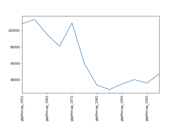
Seems the variability in this value is due to a sharp drop after 1972. Some geopolitics at play perhaps? Given the dominance of oil producing countries, maybe the Brent crude index would make an interesting comparison? Whilst Myanmar consistently has the lowest GDP, the highest GDP nation has varied more notably.

More Correlations

This short program creates a plot showing the correlation between GDP and life expectancy for 2007, normalizing marker size by population:

PYTHON

data_all = pd.read_csv('data/gapminder_all.csv', index_col='country')
data_all.plot(kind='scatter', x='gdpPercap_2007', y='lifeExp_2007',
              s=data_all['pop_2007']/1e6)

Using online help and other resources, explain what each argument to plot does.

Show me the solution

A good place to look is the documentation for the plot function - help(data_all.plot).

kind - As seen already this determines the kind of plot to be drawn.

x and y - A column name or index that determines what data will be placed on the x and y axes of the plot

s - Details for this can be found in the documentation of plt.scatter. A single number or one value for each data point. Determines the size of the plotted points.

Saving your plot to a file

If you are satisfied with the plot you see you may want to save it to a file, perhaps to include it in a publication. There is a function in the matplotlib.pyplot module that accomplishes this: savefig. Calling this function, e.g. with

PYTHON

plt.savefig('my_figure.png')

will save the current figure to the file my_figure.png. The file format will automatically be deduced from the file name extension (other formats are pdf, ps, eps and svg).

Note that functions in plt refer to a global figure variable and after a figure has been displayed to the screen (e.g. with plt.show) matplotlib will make this variable refer to a new empty figure. Therefore, make sure you call plt.savefig before the plot is displayed to the screen, otherwise you may find a file with an empty plot.

When using dataframes, data is often generated and plotted to screen in one line. In addition to using plt.savefig, we can save a reference to the current figure in a local variable (with plt.gcf) and call the savefig class method from that variable to save the figure to file.

PYTHON

data.plot(kind='bar')
fig = plt.gcf() # get current figure
fig.savefig('my_figure.png')

Making your plots accessible

Whenever you are generating plots to go into a paper or a presentation, there are a few things you can do to make sure that everyone can understand your plots.

Always make sure your text is large enough to read. Use the fontsize parameter in xlabel, ylabel, title, and legend, and tick_params with labelsize to increase the text size of the numbers on your axes.
Similarly, you should make your graph elements easy to see. Use s to increase the size of your scatterplot markers and linewidth to increase the sizes of your plot lines.
Using color (and nothing else) to distinguish between different plot elements will make your plots unreadable to anyone who is colorblind, or who happens to have a black-and-white office printer. For lines, the linestyle parameter lets you use different types of lines. For scatterplots, marker lets you change the shape of your points. If you’re unsure about your colors, you can use Coblis or Color Oracle to simulate what your plots would look like to those with colorblindness.

Key Points

matplotlib is the most widely used scientific plotting library in Python.
Plot data directly from a Pandas dataframe.
Select and transform data, then plot it.
Many styles of plot are available: see the Python Graph Gallery for more options.
Can plot many sets of data together.

Content from Lunch

Last updated on 2023-05-02 | Edit this page

Over lunch, reflect on and discuss the following:

What sort of packages might you use in Python and why would you use them?
How would data need to be formatted to be used in Pandas data frames? Would the data you have meet these requirements?
What limitations or problems might you run into when thinking about how to apply what we’ve learned to your own projects or data?

Content from Lists

Last updated on 2023-07-24 | Edit this page

Overview

Questions

How can I store multiple values?

Objectives

Explain why programs need collections of values.
Write programs that create flat lists, index them, slice them, and modify them through assignment and method calls.

A list stores many values in a single structure.

Doing calculations with a hundred variables called pressure_001, pressure_002, etc., would be at least as slow as doing them by hand.
Use a list to store many values together.
- Contained within square brackets [...].
- Values separated by commas ,.
Use len to find out how many values are in a list.

PYTHON

pressures = [0.273, 0.275, 0.277, 0.275, 0.276]
print('pressures:', pressures)
print('length:', len(pressures))

OUTPUT

pressures: [0.273, 0.275, 0.277, 0.275, 0.276]
length: 5

Use an item’s index to fetch it from a list.

Just like strings.

PYTHON

print('zeroth item of pressures:', pressures[0])
print('fourth item of pressures:', pressures[4])

OUTPUT

zeroth item of pressures: 0.273
fourth item of pressures: 0.276

Lists’ values can be replaced by assigning to them.

Use an index expression on the left of assignment to replace a value.

PYTHON

pressures[0] = 0.265
print('pressures is now:', pressures)

OUTPUT

pressures is now: [0.265, 0.275, 0.277, 0.275, 0.276]

Appending items to a list lengthens it.

Use list_name.append to add items to the end of a list.

PYTHON

primes = [2, 3, 5]
print('primes is initially:', primes)
primes.append(7)
print('primes has become:', primes)

OUTPUT

primes is initially: [2, 3, 5]
primes has become: [2, 3, 5, 7]

append is a method of lists.
- Like a function, but tied to a particular object.
Use object_name.method_name to call methods.
- Deliberately resembles the way we refer to things in a library.
We will meet other methods of lists as we go along.
- Use help(list) for a preview.
extend is similar to append, but it allows you to combine two lists. For example:

PYTHON

teen_primes = [11, 13, 17, 19]
middle_aged_primes = [37, 41, 43, 47]
print('primes is currently:', primes)
primes.extend(teen_primes)
print('primes has now become:', primes)
primes.append(middle_aged_primes)
print('primes has finally become:', primes)

OUTPUT

primes is currently: [2, 3, 5, 7]
primes has now become: [2, 3, 5, 7, 11, 13, 17, 19]
primes has finally become: [2, 3, 5, 7, 11, 13, 17, 19, [37, 41, 43, 47]]

Note that while extend maintains the “flat” structure of the list, appending a list to a list means the last element in primes will itself be a list, not an integer. Lists can contain values of any type; therefore, lists of lists are possible.

Use `del` to remove items from a list entirely.

We use del list_name[index] to remove an element from a list (in the example, 9 is not a prime number) and thus shorten it.
del is not a function or a method, but a statement in the language.

PYTHON

primes = [2, 3, 5, 7, 9]
print('primes before removing last item:', primes)
del primes[4]
print('primes after removing last item:', primes)

OUTPUT

primes before removing last item: [2, 3, 5, 7, 9]
primes after removing last item: [2, 3, 5, 7]

The empty list contains no values.

Use [] on its own to represent a list that doesn’t contain any values.
- “The zero of lists.”
Helpful as a starting point for collecting values (which we will see in the next episode).

Lists may contain values of different types.

A single list may contain numbers, strings, and anything else.

PYTHON

goals = [1, 'Create lists.', 2, 'Extract items from lists.', 3, 'Modify lists.']

Character strings can be indexed like lists.

Get single characters from a character string using indexes in square brackets.

PYTHON

element = 'carbon'
print('zeroth character:', element[0])
print('third character:', element[3])

OUTPUT

zeroth character: c
third character: b

Character strings are immutable.

Cannot change the characters in a string after it has been created.
- Immutable: can’t be changed after creation.
- In contrast, lists are mutable: they can be modified in place.
Python considers the string to be a single value with parts, not a collection of values.

PYTHON

element[0] = 'C'

ERROR

TypeError: 'str' object does not support item assignment

Lists and character strings are both collections.

Indexing beyond the end of the collection is an error.

Python reports an IndexError if we attempt to access a value that doesn’t exist.
- This is a kind of runtime error.
- Cannot be detected as the code is parsed because the index might be calculated based on data.

PYTHON

print('99th element of element is:', element[99])

OUTPUT

IndexError: string index out of range

Fill in the Blanks

Fill in the blanks so that the program below produces the output shown.

PYTHON

values = ____
values.____(1)
values.____(3)
values.____(5)
print('first time:', values)
values = values[____]
print('second time:', values)

OUTPUT

first time: [1, 3, 5]
second time: [3, 5]

Show me the solution

PYTHON

values = []
values.append(1)
values.append(3)
values.append(5)
print('first time:', values)
values = values[1:]
print('second time:', values)

How Large is a Slice?

If start and stop are both non-negative integers, how long is the list values[start:stop]?

Show me the solution

The list values[start:stop] has up to stop - start elements. For example, values[1:4] has the 3 elements values[1], values[2], and values[3]. Why ‘up to’? As we saw in episode 2, if stop is greater than the total length of the list values, we will still get a list back but it will be shorter than expected.

From Strings to Lists and Back

Given this:

PYTHON

print('string to list:', list('tin'))
print('list to string:', ''.join(['g', 'o', 'l', 'd']))

OUTPUT

string to list: ['t', 'i', 'n']
list to string: gold

What does list('some string') do?
What does '-'.join(['x', 'y', 'z']) generate?

Show me the solution

list('some string') converts a string into a list containing all of its characters.
join returns a string that is the concatenation of each string element in the list and adds the separator between each element in the list. This results in x-y-z. The separator between the elements is the string that provides this method.

Working With the End

What does the following program print?

PYTHON

element = 'helium'
print(element[-1])

How does Python interpret a negative index?
If a list or string has N elements, what is the most negative index that can safely be used with it, and what location does that index represent?
If values is a list, what does del values[-1] do?
How can you display all elements but the last one without changing values? (Hint: you will need to combine slicing and negative indexing.)

Show me the solution

The program prints m.

Python interprets a negative index as starting from the end (as opposed to starting from the beginning). The last element is -1.
The last index that can safely be used with a list of N elements is element -N, which represents the first element.
del values[-1] removes the last element from the list.
values[:-1]

Stepping Through a List

What does the following program print?

PYTHON

element = 'fluorine'
print(element[::2])
print(element[::-1])

If we write a slice as low:high:stride, what does stride do?
What expression would select all of the even-numbered items from a collection?

Show me the solution

The program prints

PYTHON

furn
eniroulf

stride is the step size of the slice.
The slice 1::2 selects all even-numbered items from a collection: it starts with element 1 (which is the second element, since indexing starts at 0), goes on until the end (since no end is given), and uses a step size of 2 (i.e., selects every second element).

Slice Bounds

What does the following program print?

PYTHON

element = 'lithium'
print(element[0:20])
print(element[-1:3])

Show me the solution

OUTPUT

lithium

The first statement prints the whole string, since the slice goes beyond the total length of the string. The second statement returns an empty string, because the slice goes “out of bounds” of the string.

Sort and Sorted

What do these two programs print? In simple terms, explain the difference between sorted(letters) and letters.sort().

PYTHON

# Program A
letters = list('gold')
result = sorted(letters)
print('letters is', letters, 'and result is', result)

PYTHON

# Program B
letters = list('gold')
result = letters.sort()
print('letters is', letters, 'and result is', result)

Show me the solution

Program A prints

OUTPUT

letters is ['g', 'o', 'l', 'd'] and result is ['d', 'g', 'l', 'o']

Program B prints

OUTPUT

letters is ['d', 'g', 'l', 'o'] and result is None

sorted(letters) returns a sorted copy of the list letters (the original list letters remains unchanged), while letters.sort() sorts the list letters in-place and does not return anything.

Copying (or Not)

What do these two programs print? In simple terms, explain the difference between new = old and new = old[:].

PYTHON

# Program A
old = list('gold')
new = old      # simple assignment
new[0] = 'D'
print('new is', new, 'and old is', old)

PYTHON

# Program B
old = list('gold')
new = old[:]   # assigning a slice
new[0] = 'D'
print('new is', new, 'and old is', old)

Show me the solution

Program A prints

OUTPUT

new is ['D', 'o', 'l', 'd'] and old is ['D', 'o', 'l', 'd']

Program B prints

OUTPUT

new is ['D', 'o', 'l', 'd'] and old is ['g', 'o', 'l', 'd']

new = old makes new a reference to the list old; new and old point towards the same object.

new = old[:] however creates a new list object new containing all elements from the list old; new and old are different objects.

Key Points

A list stores many values in a single structure.
Use an item’s index to fetch it from a list.
Lists’ values can be replaced by assigning to them.
Appending items to a list lengthens it.
Use del to remove items from a list entirely.
The empty list contains no values.
Lists may contain values of different types.
Character strings can be indexed like lists.
Character strings are immutable.
Indexing beyond the end of the collection is an error.

Content from For Loops

Last updated on 2023-05-02 | Edit this page

Overview

Questions

How can I make a program do many things?

Objectives

Explain what for loops are normally used for.
Trace the execution of a simple (unnested) loop and correctly state the values of variables in each iteration.
Write for loops that use the Accumulator pattern to aggregate values.

A for loop executes commands once for each value in a collection.

Doing calculations on the values in a list one by one is as painful as working with pressure_001, pressure_002, etc.
A for loop tells Python to execute some statements once for each value in a list, a character string, or some other collection.
“for each thing in this group, do these operations”

PYTHON

for number in [2, 3, 5]:
    print(number)

This for loop is equivalent to:

PYTHON

print(2)
print(3)
print(5)

And the for loop’s output is:

OUTPUT

2
3
5

A `for` loop is made up of a collection, a loop variable, and a body.

PYTHON

for number in [2, 3, 5]:
    print(number)

The collection, [2, 3, 5], is what the loop is being run on.
The body, print(number), specifies what to do for each value in the collection.
The loop variable, number, is what changes for each iteration of the loop.
- The “current thing”.

The first line of the `for` loop must end with a colon, and the body must be indented.

The colon at the end of the first line signals the start of a block of statements.
Python uses indentation rather than {} or begin/end to show nesting.
- Any consistent indentation is legal, but almost everyone uses four spaces.

PYTHON

for number in [2, 3, 5]:
print(number)

ERROR

IndentationError: expected an indented block

Indentation is always meaningful in Python.

PYTHON

firstName = "Jon"
  lastName = "Smith"

ERROR

  File "<ipython-input-7-f65f2962bf9c>", line 2
    lastName = "Smith"
    ^
IndentationError: unexpected indent

This error can be fixed by removing the extra spaces at the beginning of the second line.

Loop variables can be called anything.

As with all variables, loop variables are:
- Created on demand.
- Meaningless: their names can be anything at all.

PYTHON

for kitten in [2, 3, 5]:
    print(kitten)

The body of a loop can contain many statements.

But no loop should be more than a few lines long.
Hard for human beings to keep larger chunks of code in mind.

PYTHON

primes = [2, 3, 5]
for p in primes:
    squared = p ** 2
    cubed = p ** 3
    print(p, squared, cubed)

OUTPUT

2 4 8
3 9 27
5 25 125

Use `range` to iterate over a sequence of numbers.

The built-in function range produces a sequence of numbers.
- Not a list: the numbers are produced on demand to make looping over large ranges more efficient.
range(N) is the numbers 0..N-1
- Exactly the legal indices of a list or character string of length N

PYTHON

print('a range is not a list: range(0, 3)')
for number in range(0, 3):
    print(number)

OUTPUT

a range is not a list: range(0, 3)
0
1
2

The Accumulator pattern turns many values into one.

A common pattern in programs is to:
1. Initialize an accumulator variable to zero, the empty string, or the empty list.
2. Update the variable with values from a collection.

PYTHON

# Sum the first 10 integers.
total = 0
for number in range(10):
   total = total + (number + 1)
print(total)

OUTPUT

Read total = total + (number + 1) as:
- Add 1 to the current value of the loop variable number.
- Add that to the current value of the accumulator variable total.
- Assign that to total, replacing the current value.
We have to add number + 1 because range produces 0..9, not 1..10.

Classifying Errors

Is an indentation error a syntax error or a runtime error?

Show me the solution

An IndentationError is a syntax error. Programs with syntax errors cannot be started. A program with a runtime error will start but an error will be thrown under certain conditions.

Tracing Execution

Create a table showing the numbers of the lines that are executed when this program runs, and the values of the variables after each line is executed.

PYTHON

total = 0
for char in "tin":
    total = total + 1

Show me the solution

Line no	Variables
1	total = 0
2	total = 0 char = ‘t’
3	total = 1 char = ‘t’
2	total = 1 char = ‘i’
3	total = 2 char = ‘i’
2	total = 2 char = ‘n’
3	total = 3 char = ‘n’

Reversing a String

Fill in the blanks in the program below so that it prints “nit” (the reverse of the original character string “tin”).

PYTHON

original = "tin"
result = ____
for char in original:
    result = ____
print(result)

Show me the solution

PYTHON

original = "tin"
result = ""
for char in original:
    result = char + result
print(result)

Practice Accumulating

Fill in the blanks in each of the programs below to produce the indicated result.

PYTHON

# Total length of the strings in the list: ["red", "green", "blue"] => 12
total = 0
for word in ["red", "green", "blue"]:
    ____ = ____ + len(word)
print(total)

Show me the solution

PYTHON

total = 0
for word in ["red", "green", "blue"]:
    total = total + len(word)
print(total)

Practice Accumulating (continued)

PYTHON

# List of word lengths: ["red", "green", "blue"] => [3, 5, 4]
lengths = ____
for word in ["red", "green", "blue"]:
    lengths.____(____)
print(lengths)

Show me the solution

PYTHON

lengths = []
for word in ["red", "green", "blue"]:
    lengths.append(len(word))
print(lengths)

Practice Accumulating (continued)

PYTHON

# Concatenate all words: ["red", "green", "blue"] => "redgreenblue"
words = ["red", "green", "blue"]
result = ____
for ____ in ____:
    ____
print(result)

Show me the solution

PYTHON

words = ["red", "green", "blue"]
result = ""
for word in words:
    result = result + word
print(result)

Practice Accumulating (continued)

Create an acronym: Starting from the list ["red", "green", "blue"], create the acronym "RGB" using a for loop.

Hint: You may need to use a string method to properly format the acronym.

Show me the solution

PYTHON

acronym = ""
for word in ["red", "green", "blue"]:
    acronym = acronym + word[0].upper()
print(acronym)

Cumulative Sum

Reorder and properly indent the lines of code below so that they print a list with the cumulative sum of data. The result should be [1, 3, 5, 10].

PYTHON

cumulative.append(total)
for number in data:
cumulative = []
total = total + number
total = 0
print(cumulative)
data = [1,2,2,5]

Show me the solution

PYTHON

total = 0
data = [1,2,2,5]
cumulative = []
for number in data:
    total = total + number
    cumulative.append(total)
print(cumulative)

Identifying Variable Name Errors

Read the code below and try to identify what the errors are without running it.
Run the code and read the error message. What type of NameError do you think this is? Is it a string with no quotes, a misspelled variable, or a variable that should have been defined but was not?
Fix the error.
Repeat steps 2 and 3, until you have fixed all the errors.

PYTHON

for number in range(10):
    # use a if the number is a multiple of 3, otherwise use b
    if (Number % 3) == 0:
        message = message + a
    else:
        message = message + "b"
print(message)

Show me the solution

Python variable names are case sensitive: number and Number refer to different variables.
The variable message needs to be initialized as an empty string.
We want to add the string "a" to message, not the undefined variable a.

PYTHON

message = ""
for number in range(10):
    # use a if the number is a multiple of 3, otherwise use b
    if (number % 3) == 0:
        message = message + "a"
    else:
        message = message + "b"
print(message)

Identifying Item Errors

Read the code below and try to identify what the errors are without running it.
Run the code, and read the error message. What type of error is it?
Fix the error.

PYTHON

seasons = ['Spring', 'Summer', 'Fall', 'Winter']
print('My favorite season is ', seasons[4])

Show me the solution

This list has 4 elements and the index to access the last element in the list is 3.

PYTHON

seasons = ['Spring', 'Summer', 'Fall', 'Winter']
print('My favorite season is ', seasons[3])

Key Points

A for loop executes commands once for each value in a collection.
A for loop is made up of a collection, a loop variable, and a body.
The first line of the for loop must end with a colon, and the body must be indented.
Indentation is always meaningful in Python.
Loop variables can be called anything (but it is strongly advised to have a meaningful name to the looping variable).
The body of a loop can contain many statements.
Use range to iterate over a sequence of numbers.
The Accumulator pattern turns many values into one.

Content from Conditionals

Last updated on 2024-02-16 | Edit this page

Overview

Questions

How can programs do different things for different data?

Objectives

Correctly write programs that use if and else statements and simple Boolean expressions (without logical operators).
Trace the execution of unnested conditionals and conditionals inside loops.

Use `if` statements to control whether or not a block of code is executed.

An if statement (more properly called a conditional statement) controls whether some block of code is executed or not.
Structure is similar to a for statement:
- First line opens with if and ends with a colon
- Body containing one or more statements is indented (usually by 4 spaces)

PYTHON

mass = 3.54
if mass > 3.0:
    print(mass, 'is large')

mass = 2.07
if mass > 3.0:
    print (mass, 'is large')

OUTPUT

3.54 is large

Conditionals are often used inside loops.

Not much point using a conditional when we know the value (as above).
But useful when we have a collection to process.

PYTHON

masses = [3.54, 2.07, 9.22, 1.86, 1.71]
for m in masses:
    if m > 3.0:
        print(m, 'is large')

OUTPUT

3.54 is large
9.22 is large

Use `else` to execute a block of code when an `if` condition is not true.

else can be used following an if.
Allows us to specify an alternative to execute when the if branch isn’t taken.

PYTHON

masses = [3.54, 2.07, 9.22, 1.86, 1.71]
for m in masses:
    if m > 3.0:
        print(m, 'is large')
    else:
        print(m, 'is small')

OUTPUT

3.54 is large
2.07 is small
9.22 is large
1.86 is small
1.71 is small

Use `elif` to specify additional tests.

May want to provide several alternative choices, each with its own test.
Use elif (short for “else if”) and a condition to specify these.
Always associated with an if.
Must come before the else (which is the “catch all”).

PYTHON

masses = [3.54, 2.07, 9.22, 1.86, 1.71]
for m in masses:
    if m > 9.0:
        print(m, 'is HUGE')
    elif m > 3.0:
        print(m, 'is large')
    else:
        print(m, 'is small')

OUTPUT

3.54 is large
2.07 is small
9.22 is HUGE
1.86 is small
1.71 is small

Conditions are tested once, in order.

Python steps through the branches of the conditional in order, testing each in turn.
So ordering matters.

PYTHON

grade = 85
if grade >= 90:
    print('grade is A')
elif grade >= 80:
    print('grade is B')
elif grade >= 70:
    print('grade is C')

OUTPUT

grade is B

Does not automatically go back and re-evaluate if values change.

PYTHON

velocity = 10.0
if velocity > 20.0:
    print('moving too fast')
else:
    print('adjusting velocity')
    velocity = 50.0

OUTPUT

adjusting velocity

Often use conditionals in a loop to “evolve” the values of variables.

PYTHON

velocity = 10.0
for i in range(5): # execute the loop 5 times
    print(i, ':', velocity)
    if velocity > 20.0:
        print('moving too fast')
        velocity = velocity - 5.0
    else:
        print('moving too slow')
        velocity = velocity + 10.0
print('final velocity:', velocity)

OUTPUT

0 : 10.0
moving too slow
1 : 20.0
moving too slow
2 : 30.0
moving too fast
3 : 25.0
moving too fast
4 : 20.0
moving too slow
final velocity: 30.0

Create a table showing variables’ values to trace a program’s execution.

i	0	.	1	.	2	.	3	.	4	.
velocity	10.0	20.0	.	30.0	.	25.0	.	20.0	.	30.0

The program must have a print statement outside the body of the loop to show the final value of velocity, since its value is updated by the last iteration of the loop.

Compound Relations Using `and`, `or`, and Parentheses

Often, you want some combination of things to be true. You can combine relations within a conditional using and and or. Continuing the example above, suppose you have

PYTHON

mass     = [ 3.54,  2.07,  9.22,  1.86,  1.71]
velocity = [10.00, 20.00, 30.00, 25.00, 20.00]

i = 0
for i in range(5):
    if mass[i] > 5 and velocity[i] > 20:
        print("Fast heavy object.  Duck!")
    elif mass[i] > 2 and mass[i] <= 5 and velocity[i] <= 20:
        print("Normal traffic")
    elif mass[i] <= 2 and velocity[i] <= 20:
        print("Slow light object.  Ignore it")
    else:
        print("Whoa!  Something is up with the data.  Check it")

Just like with arithmetic, you can and should use parentheses whenever there is possible ambiguity. A good general rule is to always use parentheses when mixing and and or in the same condition. That is, instead of:

PYTHON

if mass[i] <= 2 or mass[i] >= 5 and velocity[i] > 20:

write one of these:

PYTHON

if (mass[i] <= 2 or mass[i] >= 5) and velocity[i] > 20:
if mass[i] <= 2 or (mass[i] >= 5 and velocity[i] > 20):

so it is perfectly clear to a reader (and to Python) what you really mean.

Tracing Execution

What does this program print?

PYTHON

pressure = 71.9
if pressure > 50.0:
    pressure = 25.0
elif pressure <= 50.0:
    pressure = 0.0
print(pressure)

Show me the solution

OUTPUT

25.0

Trimming Values

Fill in the blanks so that this program creates a new list containing zeroes where the original list’s values were negative and ones where the original list’s values were positive.

PYTHON

original = [-1.5, 0.2, 0.4, 0.0, -1.3, 0.4]
result = ____
for value in original:
    if ____:
        result.append(0)
    else:
        ____
print(result)

OUTPUT

[0, 1, 1, 1, 0, 1]

Show me the solution

PYTHON

original = [-1.5, 0.2, 0.4, 0.0, -1.3, 0.4]
result = []
for value in original:
    if value < 0.0:
        result.append(0)
    else:
        result.append(1)
print(result)

Processing Small Files

Modify this program so that it only processes files with fewer than 50 records.

PYTHON

import glob
import pandas as pd
for filename in glob.glob('data/*.csv'):
    contents = pd.read_csv(filename)
    ____:
        print(filename, len(contents))

Show me the solution

PYTHON

import glob
import pandas as pd
for filename in glob.glob('data/*.csv'):
    contents = pd.read_csv(filename)
    if len(contents) < 50:
        print(filename, len(contents))

Initializing

Modify this program so that it finds the largest and smallest values in the list no matter what the range of values originally is.

PYTHON

values = [...some test data...]
smallest, largest = None, None
for v in values:
    if ____:
        smallest, largest = v, v
    ____:
        smallest = min(____, v)
        largest = max(____, v)
print(smallest, largest)

What are the advantages and disadvantages of using this method to find the range of the data?

Show me the solution

PYTHON

values = [-2,1,65,78,-54,-24,100]
smallest, largest = None, None
for v in values:
    if smallest is None and largest is None:
        smallest, largest = v, v
    else:
        smallest = min(smallest, v)
        largest = max(largest, v)
print(smallest, largest)

If you wrote == None instead of is None, that works too, but Python programmers always write is None because of the special way None works in the language.

It can be argued that an advantage of using this method would be to make the code more readable. However, a disadvantage is that this code is not efficient because within each iteration of the for loop statement, there are two more loops that run over two numbers each (the min and max functions). It would be more efficient to iterate over each number just once:

PYTHON

values = [-2,1,65,78,-54,-24,100]
smallest, largest = None, None
for v in values:
    if smallest is None or v < smallest:
        smallest = v
    if largest is None or v > largest:
        largest = v
print(smallest, largest)

Now we have one loop, but four comparison tests. There are two ways we could improve it further: either use fewer comparisons in each iteration, or use two loops that each contain only one comparison test. The simplest solution is often the best:

PYTHON

values = [-2,1,65,78,-54,-24,100]
smallest = min(values)
largest = max(values)
print(smallest, largest)

Key Points

Use if statements to control whether or not a block of code is executed.
Conditionals are often used inside loops.
Use else to execute a block of code when an if condition is not true.
Use elif to specify additional tests.
Conditions are tested once, in order.
Create a table showing variables’ values to trace a program’s execution.

Content from Looping Over Data Sets

Last updated on 2024-12-03 | Edit this page

Overview

Questions

How can I process many data sets with a single command?

Objectives

Be able to read and write globbing expressions that match sets of files.
Use glob to create lists of files.
Write for loops to perform operations on files given their names in a list.

Use a `for` loop to process files given a list of their names.

A filename is a character string.
And lists can contain character strings.

PYTHON

import pandas as pd
for filename in ['data/gapminder_gdp_africa.csv', 'data/gapminder_gdp_asia.csv']:
    data = pd.read_csv(filename, index_col='country')
    print(filename, data.min())

OUTPUT

data/gapminder_gdp_africa.csv gdpPercap_1952    298.846212
gdpPercap_1957    335.997115
gdpPercap_1962    355.203227
gdpPercap_1967    412.977514
⋮ ⋮ ⋮
gdpPercap_1997    312.188423
gdpPercap_2002    241.165877
gdpPercap_2007    277.551859
dtype: float64
data/gapminder_gdp_asia.csv gdpPercap_1952    331
gdpPercap_1957    350
gdpPercap_1962    388
gdpPercap_1967    349
⋮ ⋮ ⋮
gdpPercap_1997    415
gdpPercap_2002    611
gdpPercap_2007    944
dtype: float64

Use `glob.glob` to find sets of files whose names match a pattern.

In Unix, the term “globbing” means “matching a set of files with a pattern”.
The most common patterns are:
- * meaning “match zero or more characters”
- ? meaning “match exactly one character”
Python’s standard library contains the glob module to provide pattern matching functionality
The glob module contains a function also called glob to match file patterns
E.g., glob.glob('*.txt') matches all files in the current directory whose names end with .txt.
Result is a (possibly empty) list of character strings.

PYTHON

import glob
print('all csv files in data directory:', glob.glob('data/*.csv'))

OUTPUT

all csv files in data directory: ['data/gapminder_all.csv', 'data/gapminder_gdp_africa.csv', \
'data/gapminder_gdp_americas.csv', 'data/gapminder_gdp_asia.csv', 'data/gapminder_gdp_europe.csv', \
'data/gapminder_gdp_oceania.csv']

PYTHON

print('all PDB files:', glob.glob('*.pdb'))

OUTPUT

all PDB files: []

Use `glob` and `for` to process batches of files.

Helps a lot if the files are named and stored systematically and consistently so that simple patterns will find the right data.

PYTHON

for filename in glob.glob('data/gapminder_*.csv'):
    data = pd.read_csv(filename)
    print(filename, data['gdpPercap_1952'].min())

OUTPUT

data/gapminder_all.csv 298.8462121
data/gapminder_gdp_africa.csv 298.8462121
data/gapminder_gdp_americas.csv 1397.717137
data/gapminder_gdp_asia.csv 331.0
data/gapminder_gdp_europe.csv 973.5331948
data/gapminder_gdp_oceania.csv 10039.59564

This includes all data, as well as per-region data.
Use a more specific pattern in the exercises to exclude the whole data set.
But note that the minimum of the entire data set is also the minimum of one of the data sets, which is a nice check on correctness.

Determining Matches

Which of these files is not matched by the expression glob.glob('data/*as*.csv')?

data/gapminder_gdp_africa.csv
data/gapminder_gdp_americas.csv
data/gapminder_gdp_asia.csv

Show me the solution

1 is not matched by the glob.

Minimum File Size

Modify this program so that it prints the number of records in the file that has the fewest records.

PYTHON

import glob
import pandas as pd
fewest = ____
for filename in glob.glob('data/*.csv'):
    dataframe = pd.____(filename)
    fewest = min(____, dataframe.shape[0])
print('smallest file has', fewest, 'records')

Note that the DataFrame.shape() method returns a tuple with the number of rows and columns of the data frame.

Show me the solution

PYTHON

import glob
import pandas as pd
fewest = float('Inf')
for filename in glob.glob('data/*.csv'):
    dataframe = pd.read_csv(filename)
    fewest = min(fewest, dataframe.shape[0])
print('smallest file has', fewest, 'records')

You might have chosen to initialize the fewest variable with a number greater than the numbers you’re dealing with, but that could lead to trouble if you reuse the code with bigger numbers. Python lets you use positive infinity, which will work no matter how big your numbers are. What other special strings does the float function recognize?

Comparing Data

Write a program that reads in the regional data sets and plots the average GDP per capita for each region over time in a single chart. Pandas will raise an error if it encounters non-numeric columns in a dataframe computation so you may need to either filter out those columns or tell pandas to ignore them.

Show me the solution

This solution builds a useful legend by using the string split method to extract the region from the path ‘data/gapminder_gdp_a_specific_region.csv’.

PYTHON

import glob
import pandas as pd
import matplotlib.pyplot as plt
fig, ax = plt.subplots(1,1)
for filename in glob.glob('data/gapminder_gdp*.csv'):
    dataframe = pd.read_csv(filename)
    # extract <region> from the filename, expected to be in the format 'data/gapminder_gdp_<region>.csv'.
    # we will split the string using the split method and `_` as our separator,
    # retrieve the last string in the list that split returns (`<region>.csv`), 
    # and then remove the `.csv` extension from that string.
    # NOTE: the pathlib module covered in the next callout also offers
    # convenient abstractions for working with filesystem paths and could solve this as well:
    # from pathlib import Path
    # region = Path(filename).stem.split('_')[-1]
    region = filename.split('_')[-1][:-4]
    # extract the years from the columns of the dataframe 
    headings = dataframe.columns[1:]
    years = headings.str.split('_').str.get(1)
    # pandas raises errors when it encounters non-numeric columns in a dataframe computation
    # but we can tell pandas to ignore them with the `numeric_only` parameter
    dataframe.mean(numeric_only=True).plot(ax=ax, label=region)
    # NOTE: another way of doing this selects just the columns with gdp in their name using the filter method
    # dataframe.filter(like="gdp").mean().plot(ax=ax, label=region)
# set the title and labels
ax.set_title('GDP Per Capita for Regions Over Time')
ax.set_xticks(range(len(years)))
ax.set_xticklabels(years)
ax.set_xlabel('Year')
plt.tight_layout()
plt.legend()
plt.show()

Dealing with File Paths

The pathlib module provides useful abstractions for file and path manipulation like returning the name of a file without the file extension. This is very useful when looping over files and directories. In the example below, we create a Path object and inspect its attributes.

PYTHON

from pathlib import Path

p = Path("data/gapminder_gdp_africa.csv")
print(p.parent)
print(p.stem)
print(p.suffix)

OUTPUT

data
gapminder_gdp_africa
.csv

Hint: Check all available attributes and methods on the Path object with the dir() function.

Key Points

Use a for loop to process files given a list of their names.
Use glob.glob to find sets of files whose names match a pattern.
Use glob and for to process batches of files.

Content from Afternoon Coffee

Last updated on 2023-05-02 | Edit this page

Reflection exercise

Over break, reflect on and discuss the following:

A common refrain in software engineering is “Don’t Repeat Yourself”. How do the techniques we’ve learned in the last lessons help us avoid repeating ourselves? Note that in practice there is some nuance to this and should be balanced with doing the simplest thing that could possibly work.
What are the pros / cons of making a variable global or local to a function?
When would you consider turning a block of code into a function definition?

Content from Writing Functions

Last updated on 2024-06-13 | Edit this page

Overview

Questions

How can I create my own functions?

Objectives

Explain and identify the difference between function definition and function call.
Write a function that takes a small, fixed number of arguments and produces a single result.

Break programs down into functions to make them easier to understand.

Human beings can only keep a few items in working memory at a time.
Understand larger/more complicated ideas by understanding and combining pieces.
- Components in a machine.
- Lemmas when proving theorems.
Functions serve the same purpose in programs.
- Encapsulate complexity so that we can treat it as a single “thing”.
Also enables re-use.
- Write one time, use many times.

Define a function using `def` with a name, parameters, and a block of code.

Begin the definition of a new function with def.
Followed by the name of the function.
- Must obey the same rules as variable names.
Then parameters in parentheses.
- Empty parentheses if the function doesn’t take any inputs.
- We will discuss this in detail in a moment.
Then a colon.
Then an indented block of code.

PYTHON

def print_greeting():
    print('Hello!')
    print('The weather is nice today.')
    print('Right?')

Defining a function does not run it.

Defining a function does not run it.
- Like assigning a value to a variable.
Must call the function to execute the code it contains.

PYTHON

print_greeting()

OUTPUT

Hello!

Arguments in a function call are matched to its defined parameters.

Functions are most useful when they can operate on different data.
Specify parameters when defining a function.
- These become variables when the function is executed.
- Are assigned the arguments in the call (i.e., the values passed to the function).
- If you don’t name the arguments when using them in the call, the arguments will be matched to parameters in the order the parameters are defined in the function.

PYTHON

def print_date(year, month, day):
    joined = str(year) + '/' + str(month) + '/' + str(day)
    print(joined)

print_date(1871, 3, 19)

OUTPUT

1871/3/19

Or, we can name the arguments when we call the function, which allows us to specify them in any order and adds clarity to the call site; otherwise as one is reading the code they might forget if the second argument is the month or the day for example.

PYTHON

print_date(month=3, day=19, year=1871)

OUTPUT

1871/3/19

Via Twitter: () contains the ingredients for the function while the body contains the recipe.

Functions may return a result to their caller using `return`.

Use return ... to give a value back to the caller.
May occur anywhere in the function.
But functions are easier to understand if return occurs:
- At the start to handle special cases.
- At the very end, with a final result.

PYTHON

def average(values):
    if len(values) == 0:
        return None
    return sum(values) / len(values)

PYTHON

a = average([1, 3, 4])
print('average of actual values:', a)

OUTPUT

average of actual values: 2.6666666666666665

PYTHON

print('average of empty list:', average([]))

OUTPUT

average of empty list: None

Remember: every function returns something.
A function that doesn’t explicitly return a value automatically returns None.

PYTHON

result = print_date(1871, 3, 19)
print('result of call is:', result)

OUTPUT

1871/3/19
result of call is: None

Identifying Syntax Errors

Read the code below and try to identify what the errors are without running it.
Run the code and read the error message. Is it a SyntaxError or an IndentationError?
Fix the error.
Repeat steps 2 and 3 until you have fixed all the errors.

PYTHON

def another_function
  print("Syntax errors are annoying.")
   print("But at least python tells us about them!")
  print("So they are usually not too hard to fix.")

Show me the solution

PYTHON

def another_function():
  print("Syntax errors are annoying.")
  print("But at least Python tells us about them!")
  print("So they are usually not too hard to fix.")

Definition and Use

What does the following program print?

PYTHON

def report(pressure):
    print('pressure is', pressure)

print('calling', report, 22.5)

Show me the solution

OUTPUT

calling <function report at 0x7fd128ff1bf8> 22.5

A function call always needs parenthesis, otherwise you get memory address of the function object. So, if we wanted to call the function named report, and give it the value 22.5 to report on, we could have our function call as follows

PYTHON

print("calling")
report(22.5)

OUTPUT

calling
pressure is 22.5

Order of Operations

What’s wrong in this example?

PYTHON

result = print_time(11, 37, 59)

def print_time(hour, minute, second):
   time_string = str(hour) + ':' + str(minute) + ':' + str(second)
   print(time_string)

After fixing the problem above, explain why running this example code:

PYTHON

result = print_time(11, 37, 59)
print('result of call is:', result)

gives this output:

OUTPUT

11:37:59
result of call is: None

Why is the result of the call None?

Show me the solution

The problem with the example is that the function print_time() is defined after the call to the function is made. Python doesn’t know how to resolve the name print_time since it hasn’t been defined yet and will raise a NameError e.g., NameError: name 'print_time' is not defined
The first line of output 11:37:59 is printed by the first line of code, result = print_time(11, 37, 59) that binds the value returned by invoking print_time to the variable result. The second line is from the second print call to print the contents of the result variable.
print_time() does not explicitly return a value, so it automatically returns None.

Encapsulation

Fill in the blanks to create a function that takes a single filename as an argument, loads the data in the file named by the argument, and returns the minimum value in that data.

PYTHON

import pandas as pd

def min_in_data(____):
    data = ____
    return ____

Show me the solution

PYTHON

import pandas as pd

def min_in_data(filename):
    data = pd.read_csv(filename)
    return data.min()

Find the First

Fill in the blanks to create a function that takes a list of numbers as an argument and returns the first negative value in the list. What does your function do if the list is empty? What if the list has no negative numbers?

PYTHON

def first_negative(values):
    for v in ____:
        if ____:
            return ____

Show me the solution

PYTHON

def first_negative(values):
    for v in values:
        if v < 0:
            return v

If an empty list or a list with all positive values is passed to this function, it returns None:

PYTHON

my_list = []
print(first_negative(my_list))

OUTPUT

None

Calling by Name

Earlier we saw this function:

PYTHON

def print_date(year, month, day):
    joined = str(year) + '/' + str(month) + '/' + str(day)
    print(joined)

We saw that we can call the function using named arguments, like this:

PYTHON

print_date(day=1, month=2, year=2003)

What does print_date(day=1, month=2, year=2003) print?
When have you seen a function call like this before?
When and why is it useful to call functions this way?

Show me the solution

2003/2/1
We saw examples of using named arguments when working with the pandas library. For example, when reading in a dataset using data = pd.read_csv('data/gapminder_gdp_europe.csv', index_col='country'), the last argument index_col is a named argument.
Using named arguments can make code more readable since one can see from the function call what name the different arguments have inside the function. It can also reduce the chances of passing arguments in the wrong order, since by using named arguments the order doesn’t matter.

Encapsulation of an If/Print Block

The code below will run on a label-printer for chicken eggs. A digital scale will report a chicken egg mass (in grams) to the computer and then the computer will print a label.

PYTHON

import random
for i in range(10):

    # simulating the mass of a chicken egg
    # the (random) mass will be 70 +/- 20 grams
    mass = 70 + 20.0 * (2.0 * random.random() - 1.0)

    print(mass)

    # egg sizing machinery prints a label
    if mass >= 85:
        print("jumbo")
    elif mass >= 70:
        print("large")
    elif mass < 70 and mass >= 55:
        print("medium")
    else:
        print("small")

The if-block that classifies the eggs might be useful in other situations, so to avoid repeating it, we could fold it into a function, get_egg_label(). Revising the program to use the function would give us this:

PYTHON

# revised version
import random
for i in range(10):

    # simulating the mass of a chicken egg
    # the (random) mass will be 70 +/- 20 grams
    mass = 70 + 20.0 * (2.0 * random.random() - 1.0)

    print(mass, get_egg_label(mass))

Create a function definition for get_egg_label() that will work with the revised program above. Note that the get_egg_label() function’s return value will be important. Sample output from the above program would be 71.23 large.
A dirty egg might have a mass of more than 90 grams, and a spoiled or broken egg will probably have a mass that’s less than 50 grams. Modify your get_egg_label() function to account for these error conditions. Sample output could be 25 too light, probably spoiled.

Show me the solution

PYTHON

def get_egg_label(mass):
    # egg sizing machinery prints a label
    egg_label = "Unlabelled"
    if mass >= 90:
        egg_label = "warning: egg might be dirty"
    elif mass >= 85:
        egg_label = "jumbo"
    elif mass >= 70:
        egg_label = "large"
    elif mass < 70 and mass >= 55:
        egg_label = "medium"
    elif mass < 50:
        egg_label = "too light, probably spoiled"
    else:
        egg_label = "small"
    return egg_label

Encapsulating Data Analysis

Assume that the following code has been executed:

PYTHON

import pandas as pd

data_asia = pd.read_csv('data/gapminder_gdp_asia.csv', index_col=0)
japan = data_asia.loc['Japan']

Complete the statements below to obtain the average GDP for Japan across the years reported for the 1980s.

PYTHON

year = 1983
gdp_decade = 'gdpPercap_' + str(year // ____)
avg = (japan.loc[gdp_decade + ___] + japan.loc[gdp_decade + ___]) / 2

Abstract the code above into a single function.

PYTHON

def avg_gdp_in_decade(country, continent, year):
    data_countries = pd.read_csv('data/gapminder_gdp_'+___+'.csv',delimiter=',',index_col=0)
    ____
    ____
    ____
    return avg

How would you generalize this function if you did not know beforehand which specific years occurred as columns in the data? For instance, what if we also had data from years ending in 1 and 9 for each decade? (Hint: use the columns to filter out the ones that correspond to the decade, instead of enumerating them in the code.)

Show me the solution

The average GDP for Japan across the years reported for the 1980s is computed with:

PYTHON

year = 1983
gdp_decade = 'gdpPercap_' + str(year // 10)
avg = (japan.loc[gdp_decade + '2'] + japan.loc[gdp_decade + '7']) / 2

That code as a function is:

PYTHON

def avg_gdp_in_decade(country, continent, year):
    data_countries = pd.read_csv('data/gapminder_gdp_' + continent + '.csv', index_col=0)
    c = data_countries.loc[country]
    gdp_decade = 'gdpPercap_' + str(year // 10)
    avg = (c.loc[gdp_decade + '2'] + c.loc[gdp_decade + '7'])/2
    return avg

To obtain the average for the relevant years, we need to loop over them:

PYTHON

def avg_gdp_in_decade(country, continent, year):
    data_countries = pd.read_csv('data/gapminder_gdp_' + continent + '.csv', index_col=0)
    c = data_countries.loc[country]
    gdp_decade = 'gdpPercap_' + str(year // 10)
    total = 0.0
    num_years = 0
    for yr_header in c.index: # c's index contains reported years
        if yr_header.startswith(gdp_decade):
            total = total + c.loc[yr_header]
            num_years = num_years + 1
    return total/num_years

The function can now be called by:

PYTHON

avg_gdp_in_decade('Japan','asia',1983)

OUTPUT

20880.023800000003

Simulating a dynamical system

In mathematics, a dynamical system is a system in which a function describes the time dependence of a point in a geometrical space. A canonical example of a dynamical system is the logistic map, a growth model that computes a new population density (between 0 and 1) based on the current density. In the model, time takes discrete values 0, 1, 2, …

Define a function called logistic_map that takes two inputs: x, representing the current population (at time t), and a parameter r = 1. This function should return a value representing the state of the system (population) at time t + 1, using the mapping function:

f(t+1) = r * f(t) * [1 - f(t)]

Using a for or while loop, iterate the logistic_map function defined in part 1, starting from an initial population of 0.5, for a period of time t_final = 10. Store the intermediate results in a list so that after the loop terminates you have accumulated a sequence of values representing the state of the logistic map at times t = [0,1,...,t_final] (11 values in total). Print this list to see the evolution of the population.
Encapsulate the logic of your loop into a function called iterate that takes the initial population as its first input, the parameter t_final as its second input and the parameter r as its third input. The function should return the list of values representing the state of the logistic map at times t = [0,1,...,t_final]. Run this function for periods t_final = 100 and 1000 and print some of the values. Is the population trending toward a steady state?

Show me the solution

PYTHON

def logistic_map(x, r):
    return r * x * (1 - x)

PYTHON

initial_population = 0.5
t_final = 10
r = 1.0
population = [initial_population]

for t in range(t_final):
    population.append( logistic_map(population[t], r) )

PYTHON

def iterate(initial_population, t_final, r):
    population = [initial_population]
    for t in range(t_final):
        population.append( logistic_map(population[t], r) )
    return population

for period in (10, 100, 1000):
    population = iterate(0.5, period, 1)
    print(population[-1])

OUTPUT

0.06945089389714401
0.009395779870614648
0.0009913908614406382

The population seems to be approaching zero.

Using Functions With Conditionals in Pandas

Functions will often contain conditionals. Here is a short example that will indicate which quartile the argument is in based on hand-coded values for the quartile cut points.

PYTHON

def calculate_life_quartile(exp):
    if exp < 58.41:
        # This observation is in the first quartile
        return 1
    elif exp >= 58.41 and exp < 67.05:
        # This observation is in the second quartile
       return 2
    elif exp >= 67.05 and exp < 71.70:
        # This observation is in the third quartile
       return 3
    elif exp >= 71.70:
        # This observation is in the fourth quartile
       return 4
    else:
        # This observation has bad data
       return None

calculate_life_quartile(62.5)

OUTPUT

That function would typically be used within a for loop, but Pandas has a different, more efficient way of doing the same thing, and that is by applying a function to a dataframe or a portion of a dataframe. Here is an example, using the definition above.

PYTHON

data = pd.read_csv('data/gapminder_all.csv')
data['life_qrtl'] = data['lifeExp_1952'].apply(calculate_life_quartile)

There is a lot in that second line, so let’s take it piece by piece. On the right side of the = we start with data['lifeExp'], which is the column in the dataframe called data labeled lifExp. We use the apply() to do what it says, apply the calculate_life_quartile to the value of this column for every row in the dataframe.

Key Points

Break programs down into functions to make them easier to understand.
Define a function using def with a name, parameters, and a block of code.
Defining a function does not run it.
Arguments in a function call are matched to its defined parameters.
Functions may return a result to their caller using return.

Content from Variable Scope

Last updated on 2023-05-02 | Edit this page

Overview

Questions

How do function calls actually work?
How can I determine where errors occurred?

Objectives

Identify local and global variables.
Identify parameters as local variables.
Read a traceback and determine the file, function, and line number on which the error occurred, the type of error, and the error message.

The scope of a variable is the part of a program that can ‘see’ that variable.

There are only so many sensible names for variables.
People using functions shouldn’t have to worry about what variable names the author of the function used.
People writing functions shouldn’t have to worry about what variable names the function’s caller uses.
The part of a program in which a variable is visible is called its scope.

PYTHON

pressure = 103.9

def adjust(t):
    temperature = t * 1.43 / pressure
    return temperature

pressure is a global variable.
- Defined outside any particular function.
- Visible everywhere.
t and temperature are local variables in adjust.
- Defined in the function.
- Not visible in the main program.
- Remember: a function parameter is a variable that is automatically assigned a value when the function is called.

PYTHON

print('adjusted:', adjust(0.9))
print('temperature after call:', temperature)

OUTPUT

adjusted: 0.01238691049085659

ERROR

Traceback (most recent call last):
  File "/Users/swcarpentry/foo.py", line 8, in <module>
    print('temperature after call:', temperature)
NameError: name 'temperature' is not defined

Local and Global Variable Use

Trace the values of all variables in this program as it is executed. (Use ‘—’ as the value of variables before and after they exist.)

PYTHON

limit = 100

def clip(value):
    return min(max(0.0, value), limit)

value = -22.5
print(clip(value))

Reading Error Messages

Read the traceback below, and identify the following:

How many levels does the traceback have?
What is the file name where the error occurred?
What is the function name where the error occurred?
On which line number in this function did the error occur?
What is the type of error?
What is the error message?

ERROR

---------------------------------------------------------------------------
KeyError                                  Traceback (most recent call last)
<ipython-input-2-e4c4cbafeeb5> in <module>()
      1 import errors_02
----> 2 errors_02.print_friday_message()

/Users/ghopper/thesis/code/errors_02.py in print_friday_message()
     13
     14 def print_friday_message():
---> 15     print_message("Friday")

/Users/ghopper/thesis/code/errors_02.py in print_message(day)
      9         "sunday": "Aw, the weekend is almost over."
     10     }
---> 11     print(messages[day])
     12
     13

KeyError: 'Friday'

Show me the solution

Three levels.
errors_02.py
print_message
Line 11
KeyError. These errors occur when we are trying to look up a key that does not exist (usually in a data structure such as a dictionary). We can find more information about the KeyError and other built-in exceptions in the Python docs.
KeyError: 'Friday'

Key Points

The scope of a variable is the part of a program that can ‘see’ that variable.

Content from Programming Style

Last updated on 2023-07-29 | Edit this page

Overview

Questions

How can I make my programs more readable?
How do most programmers format their code?
How can programs check their own operation?

Objectives

Provide sound justifications for basic rules of coding style.
Refactor one-page programs to make them more readable and justify the changes.
Use Python community coding standards (PEP-8).

Coding style

A consistent coding style helps others (including our future selves) read and understand code more easily. Code is read much more often than it is written, and as the Zen of Python states, “Readability counts”. Python proposed a standard style through one of its first Python Enhancement Proposals (PEP), PEP8.

Some points worth highlighting:

document your code and ensure that assumptions, internal algorithms, expected inputs, expected outputs, etc., are clear
use clear, semantically meaningful variable names
use white-space, not tabs, to indent lines (tabs can cause problems across different text editors, operating systems, and version control systems)

Follow standard Python style in your code.

PEP8: a style guide for Python that discusses topics such as how to name variables, how to indent your code, how to structure your import statements, etc. Adhering to PEP8 makes it easier for other Python developers to read and understand your code, and to understand what their contributions should look like.
To check your code for compliance with PEP8, you can use the pycodestyle application and tools like the black code formatter can automatically format your code to conform to PEP8 and pycodestyle (a Jupyter notebook formatter also exists nb_black).
Some groups and organizations follow different style guidelines besides PEP8. For example, the Google style guide on Python makes slightly different recommendations. Google wrote an application that can help you format your code in either their style or PEP8 called yapf.
With respect to coding style, the key is consistency. Choose a style for your project be it PEP8, the Google style, or something else and do your best to ensure that you and anyone else you are collaborating with sticks to it. Consistency within a project is often more impactful than the particular style used. A consistent style will make your software easier to read and understand for others and for your future self.

Use assertions to check for internal errors.

Assertions are a simple but powerful method for making sure that the context in which your code is executing is as you expect.

PYTHON

def calc_bulk_density(mass, volume):
    '''Return dry bulk density = powder mass / powder volume.'''
    assert volume > 0
    return mass / volume

If the assertion is False, the Python interpreter raises an AssertionError runtime exception. The source code for the expression that failed will be displayed as part of the error message. To ignore assertions in your code run the interpreter with the ‘-O’ (optimize) switch. Assertions should contain only simple checks and never change the state of the program. For example, an assertion should never contain an assignment.

Use docstrings to provide builtin help.

If the first thing in a function is a character string that is not assigned directly to a variable, Python attaches it to the function, accessible via the builtin help function. This string that provides documentation is also known as a docstring.

PYTHON

def average(values):
    "Return average of values, or None if no values are supplied."

    if len(values) == 0:
        return None
    return sum(values) / len(values)

help(average)

OUTPUT

Help on function average in module __main__:

average(values)
    Return average of values, or None if no values are supplied.

Multiline Strings

Often use multiline strings for documentation. These start and end with three quote characters (either single or double) and end with three matching characters.

PYTHON

"""This string spans
multiple lines.

Blank lines are allowed."""

What Will Be Shown?

Highlight the lines in the code below that will be available as online help. Are there lines that should be made available, but won’t be? Will any lines produce a syntax error or a runtime error?

PYTHON

"Find maximum edit distance between multiple sequences."
# This finds the maximum distance between all sequences.

def overall_max(sequences):
    '''Determine overall maximum edit distance.'''

    highest = 0
    for left in sequences:
        for right in sequences:
            '''Avoid checking sequence against itself.'''
            if left != right:
                this = edit_distance(left, right)
                highest = max(highest, this)

    # Report.
    return highest

Document This

Use comments to describe and help others understand potentially unintuitive sections or individual lines of code. They are especially useful to whoever may need to understand and edit your code in the future, including yourself.

Use docstrings to document the acceptable inputs and expected outputs of a method or class, its purpose, assumptions and intended behavior. Docstrings are displayed when a user invokes the builtin help method on your method or class.

Turn the comment in the following function into a docstring and check that help displays it properly.

PYTHON

def middle(a, b, c):
    # Return the middle value of three.
    # Assumes the values can actually be compared.
    values = [a, b, c]
    values.sort()
    return values[1]

Show me the solution

PYTHON

def middle(a, b, c):
    '''Return the middle value of three.
    Assumes the values can actually be compared.'''
    values = [a, b, c]
    values.sort()
    return values[1]

Clean Up This Code

Read this short program and try to predict what it does.
Run it: how accurate was your prediction?
Refactor the program to make it more readable. Remember to run it after each change to ensure its behavior hasn’t changed.
Compare your rewrite with your neighbor’s. What did you do the same? What did you do differently, and why?

PYTHON

n = 10
s = 'et cetera'
print(s)
i = 0
while i < n:
    # print('at', j)
    new = ''
    for j in range(len(s)):
        left = j-1
        right = (j+1)%len(s)
        if s[left]==s[right]: new = new + '-'
        else: new = new + '*'
    s=''.join(new)
    print(s)
    i += 1

Show me the solution

Here’s one solution.

PYTHON

def string_machine(input_string, iterations):
    """
    Takes input_string and generates a new string with -'s and *'s
    corresponding to characters that have identical adjacent characters
    or not, respectively.  Iterates through this procedure with the resultant
    strings for the supplied number of iterations.
    """
    print(input_string)
    input_string_length = len(input_string)
    old = input_string
    for i in range(iterations):
        new = ''
        # iterate through characters in previous string
        for j in range(input_string_length):
            left = j-1
            right = (j+1) % input_string_length  # ensure right index wraps around
            if old[left] == old[right]:
                new = new + '-'
            else:
                new = new + '*'
        print(new)
        # store new string as old
        old = new     

string_machine('et cetera', 10)

OUTPUT

et cetera
*****-***
----*-*--
---*---*-
--*-*-*-*
**-------
***-----*
--**---**
*****-***
----*-*--
---*---*-

Key Points

Follow standard Python style in your code.
Use docstrings to provide builtin help.

Content from Wrap-Up

Last updated on 2023-05-02 | Edit this page

Overview

Questions

What have we learned?
What else is out there and where do I find it?

Objectives

Name and locate scientific Python community sites for software, workshops, and help.

Leslie Lamport once said, “Writing is nature’s way of showing you how sloppy your thinking is.” The same is true of programming: many things that seem obvious when we’re thinking about them turn out to be anything but when we have to explain them precisely.

Python supports a large and diverse community across academia and industry.

The Python 3 documentation covers the core language and the standard library.
PyCon is the largest annual conference for the Python community.
SciPy is a rich collection of scientific utilities. It is also the name of a series of annual conferences.
Jupyter is the home of Project Jupyter.
Pandas is the home of the Pandas data library.
Stack Overflow’s general Python section can be helpful, as well as the sections on NumPy, SciPy, and Pandas.

Key Points

Python supports a large and diverse community across academia and industry.

Content from Feedback

Last updated on 2023-05-02 | Edit this page

Overview

Questions

How did the class go?

Objectives

Gather feedback on the class

Gather feedback from participants.

Key Points

We are constantly seeking to improve this course.

Overview

Questions

Objectives

Getting Started with JupyterLab

JupyterLab? What about Jupyter notebooks?

Starting JupyterLab

macOS - Command Line

BASH

Windows Users - Command Line

BASH

Anaconda Navigator

The JupyterLab Interface

Menu Bar

Kernels

Left Sidebar

Main Work Area

Creating a Python script

Creating a Jupyter Notebook

How It’s Stored

Arranging Documents into Panels of Tabs

Show me the solution

Code vs. Text

The Notebook has Command and Edit modes.

Command Vs. Edit

Show me the solution

Use the keyboard and mouse to select and edit cells.

The Notebook will turn Markdown into pretty-printed documentation.

Markdown does most of what HTML does.

A Level-1 Heading

A Level-2 Heading (etc.)

Creating Lists in Markdown

Show me the solution

More Math

PYTHON

Show me the solution

PYTHON

Change an Existing Cell from Code to Markdown

PYTHON

Show me the solution

PYTHON

Equations

Show me the solution

Closing JupyterLab

Closing JupyterLab

Key Points

Overview

Questions

Objectives

Use variables to store values.

PYTHON

Use print to display values.

PYTHON

OUTPUT

Variables must be created before they are used.

PYTHON

ERROR

Variables Persist Between Cells

PYTHON

PYTHON

Variables can be used in calculations.

PYTHON

OUTPUT

Use an index to get a single character from a string.

PYTHON

OUTPUT

Use a slice to get a substring.

PYTHON

OUTPUT

Use the built-in function len to find the length of a string.

PYTHON

OUTPUT

Python is case-sensitive.

Use meaningful variable names.

PYTHON

Swapping Values

PYTHON

Show me the solution

OUTPUT

Predicting Values

PYTHON

Use `print` to display values.

Use the built-in function `len` to find the length of a string.

Use the built-in function `type` to find the type of a value.