Adina nicely introduced the concept of DNA sequencing in her round 2.3 post. The sequencing data that she describes comes from a platform that generates pieces of sequence (called ‘reads’) up to a few hundred bases, but quite accurate (at least 99% of the bases, i.e. the ‘letters’ are correct). I am currently working a lot with sequencing data from a different platform. This one generates very long reads (up to 20000 bases/letters), but at a cost of a much lower accuracy (80-90% accurate).
My latest data was generated by the machine in three different ‘modes’: older chemistry (C2C2), variant 1 to make longer reads (C2XL) and variant 2 that should result in even longer reads (XLXL). I was interested in determining how accurate the data actually was. The best way to do that is to compare the reads to the ‘correct’ sequence, so-called reference genome, and counting the differences. I’ll skip the details of the mapping, i.e. finding the region of the reference genome the read comes from, but the result of this mapping is a table with 13 columns. I wanted to
— extract the percentage of similarity (identity) between the read and the reference, which is in column 6
— extract the length of the read that was mapped to the reference by subtracting column 8 (end position) from column 7 (start position)
— plot the distribution of the identity percentages
— plot some more, but that I’ll skip
Plotting I do in R (but I am learning matplotlib in python ![]() ). Reading this large table in R would take a lot of time and potentially a lot of memory. So I tried to reduce the dataset before loading it (generally a wise thing to do in programming).
). Reading this large table in R would take a lot of time and potentially a lot of memory. So I tried to reduce the dataset before loading it (generally a wise thing to do in programming).
One could extract the relevant columns from the table, and save to another file, like this
cut -f 6-8 table.txt >selected_columns.txt<br />
and read in that file into R. selected_columns.txt now only contains data from three of the original 13 columns.
Alternatively, you could use awk to combine the extraction with the calculation, i.e. subtract column 7 from column 8:
awk '{print $6, $8-$7}' table.txt >selected_columns.txt
This further reduces the dataset to two columns in selected_columns.txt.
In R, the reading in of the data would then be done like this:
C2C2 =read.table(file="selected_columns.txt", sep=" ", header=FALSE)<br />
I try to avoid intermediate/temporary files, as they create copies of the data.This is bad in principle: what if one of the files changes, who can you make sure the other is updated as well? Luckily, there is a trick in R which allows you to read in data which is the result of a shell command. Here you use the ‘pipe’ function in R:
C2C2 = read.table(pipe("awk '{print $6, $8-$7}' table.txt"), sep=" ", header=FALSE)<br />
The pipe function returns the result of a shell command, in this case the awk command I designed to extract the needed columns, and subtract column 7 from column 8.
I regularly combine shell commands (cut, grep etc) with small shell-based programs (see, awk) and read the results into a program or script (R or python) for analysis this way.
I repeated this approach for all three datasets (C2C2, C2XL and XLXL) and combined all data in one plot:
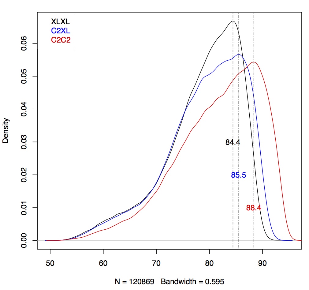
Conclusion: C2C2 data is the most accurate, followed by C2XL and XLXL (this was as expected).
Take home lesson: tools can be integrated across languages; what you learn to be convenient in language 1 (e.g., the shell) can often be used in language 2 (e.g. R or python) through a function call.