Data Frame Manipulation with tidyr
Last updated on 2024-04-04 | Edit this page
Overview
Questions
- How can I change the layout of a data frame?
Objectives
- To understand the concepts of ‘longer’ and ‘wider’ data frame
formats and be able to convert between them with
tidyr.
Researchers often want to reshape their data frames from ‘wide’ to ‘longer’ layouts, or vice-versa. The ‘long’ layout or format is where:
- each column is a variable
- each row is an observation
In the purely ‘long’ (or ‘longest’) format, you usually have 1 column for the observed variable and the other columns are ID variables.
For the ‘wide’ format each row is often a site/subject/patient and
you have multiple observation variables containing the same type of
data. These can be either repeated observations over time, or
observation of multiple variables (or a mix of both). You may find data
input may be simpler or some other applications may prefer the ‘wide’
format. However, many of R‘s functions have been designed
assuming you have ’longer’ formatted data. This tutorial will help you
efficiently transform your data shape regardless of original format.
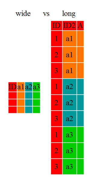
Long and wide data frame layouts mainly affect readability. For humans, the wide format is often more intuitive since we can often see more of the data on the screen due to its shape. However, the long format is more machine readable and is closer to the formatting of databases. The ID variables in our data frames are similar to the fields in a database and observed variables are like the database values.
Getting started
First install the packages if you haven’t already done so (you probably installed dplyr in the previous lesson):
R
#install.packages("tidyr")
#install.packages("dplyr")
Load the packages
R
library("tidyr")
library("dplyr")
First, lets look at the structure of our original gapminder data frame:
R
str(gapminder)
OUTPUT
'data.frame':	1704 obs. of  6 variables:
 $ country  : chr  "Afghanistan" "Afghanistan" "Afghanistan" "Afghanistan" ...
 $ year     : int  1952 1957 1962 1967 1972 1977 1982 1987 1992 1997 ...
 $ pop      : num  8425333 9240934 10267083 11537966 13079460 ...
 $ continent: chr  "Asia" "Asia" "Asia" "Asia" ...
 $ lifeExp  : num  28.8 30.3 32 34 36.1 ...
$ gdpPercap: num 779 821 853 836 740 ...The original gapminder data.frame is in an intermediate format. It is
not purely long since it had multiple observation variables
(pop,lifeExp,gdpPercap).
Sometimes, as with the gapminder dataset, we have multiple types of
observed data. It is somewhere in between the purely ‘long’ and ‘wide’
data formats. We have 3 “ID variables” (continent,
country, year) and 3 “Observation variables”
(pop,lifeExp,gdpPercap). This
intermediate format can be preferred despite not having ALL observations
in 1 column given that all 3 observation variables have different units.
There are few operations that would need us to make this data frame any
longer (i.e. 4 ID variables and 1 Observation variable).
While using many of the functions in R, which are often vector based,
you usually do not want to do mathematical operations on values with
different units. For example, using the purely long format, a single
mean for all of the values of population, life expectancy, and GDP would
not be meaningful since it would return the mean of values with 3
incompatible units. The solution is that we first manipulate the data
either by grouping (see the lesson on dplyr), or we change
the structure of the data frame. Note: Some plotting
functions in R actually work better in the wide format data.
From wide to long format with pivot_longer()
Until now, we’ve been using the nicely formatted original gapminder dataset, but ‘real’ data (i.e. our own research data) will never be so well organized. Here let’s start with the wide formatted version of the gapminder dataset.
Download the wide version of the gapminder data from this link to a csv file and save it in your data folder.
We’ll load the data file and look at it. Note: we don’t want our
continent and country columns to be factors, so we use the
stringsAsFactors argument for read.csv() to disable
that.
R
gap_wide <- read.csv("data/gapminder_wide.csv", stringsAsFactors = FALSE)
str(gap_wide)
OUTPUT
'data.frame':	142 obs. of  38 variables:
 $ continent     : chr  "Africa" "Africa" "Africa" "Africa" ...
 $ country       : chr  "Algeria" "Angola" "Benin" "Botswana" ...
 $ gdpPercap_1952: num  2449 3521 1063 851 543 ...
 $ gdpPercap_1957: num  3014 3828 960 918 617 ...
 $ gdpPercap_1962: num  2551 4269 949 984 723 ...
 $ gdpPercap_1967: num  3247 5523 1036 1215 795 ...
 $ gdpPercap_1972: num  4183 5473 1086 2264 855 ...
 $ gdpPercap_1977: num  4910 3009 1029 3215 743 ...
 $ gdpPercap_1982: num  5745 2757 1278 4551 807 ...
 $ gdpPercap_1987: num  5681 2430 1226 6206 912 ...
 $ gdpPercap_1992: num  5023 2628 1191 7954 932 ...
 $ gdpPercap_1997: num  4797 2277 1233 8647 946 ...
 $ gdpPercap_2002: num  5288 2773 1373 11004 1038 ...
 $ gdpPercap_2007: num  6223 4797 1441 12570 1217 ...
 $ lifeExp_1952  : num  43.1 30 38.2 47.6 32 ...
 $ lifeExp_1957  : num  45.7 32 40.4 49.6 34.9 ...
 $ lifeExp_1962  : num  48.3 34 42.6 51.5 37.8 ...
 $ lifeExp_1967  : num  51.4 36 44.9 53.3 40.7 ...
 $ lifeExp_1972  : num  54.5 37.9 47 56 43.6 ...
 $ lifeExp_1977  : num  58 39.5 49.2 59.3 46.1 ...
 $ lifeExp_1982  : num  61.4 39.9 50.9 61.5 48.1 ...
 $ lifeExp_1987  : num  65.8 39.9 52.3 63.6 49.6 ...
 $ lifeExp_1992  : num  67.7 40.6 53.9 62.7 50.3 ...
 $ lifeExp_1997  : num  69.2 41 54.8 52.6 50.3 ...
 $ lifeExp_2002  : num  71 41 54.4 46.6 50.6 ...
 $ lifeExp_2007  : num  72.3 42.7 56.7 50.7 52.3 ...
 $ pop_1952      : num  9279525 4232095 1738315 442308 4469979 ...
 $ pop_1957      : num  10270856 4561361 1925173 474639 4713416 ...
 $ pop_1962      : num  11000948 4826015 2151895 512764 4919632 ...
 $ pop_1967      : num  12760499 5247469 2427334 553541 5127935 ...
 $ pop_1972      : num  14760787 5894858 2761407 619351 5433886 ...
 $ pop_1977      : num  17152804 6162675 3168267 781472 5889574 ...
 $ pop_1982      : num  20033753 7016384 3641603 970347 6634596 ...
 $ pop_1987      : num  23254956 7874230 4243788 1151184 7586551 ...
 $ pop_1992      : num  26298373 8735988 4981671 1342614 8878303 ...
 $ pop_1997      : num  29072015 9875024 6066080 1536536 10352843 ...
 $ pop_2002      : int  31287142 10866106 7026113 1630347 12251209 7021078 15929988 4048013 8835739 614382 ...
 $ pop_2007      : int  33333216 12420476 8078314 1639131 14326203 8390505 17696293 4369038 10238807 710960 ...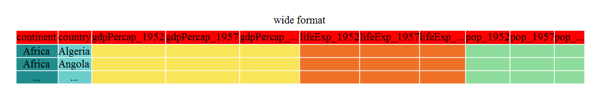
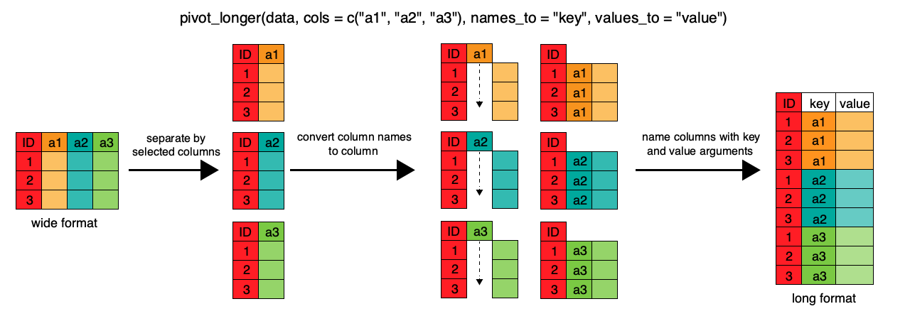
To change this very wide data frame layout back to our nice,
intermediate (or longer) layout, we will use one of the two available
pivot functions from the tidyr package. To
convert from wide to a longer format, we will use the
pivot_longer() function. pivot_longer() makes
datasets longer by increasing the number of rows and decreasing the
number of columns, or ‘lengthening’ your observation variables into a
single variable.
R
gap_long <- gap_wide %>%
  pivot_longer(
    cols = c(starts_with('pop'), starts_with('lifeExp'), starts_with('gdpPercap')),
    names_to = "obstype_year", values_to = "obs_values"
  )
str(gap_long)
OUTPUT
tibble [5,112 × 4] (S3: tbl_df/tbl/data.frame)
 $ continent   : chr [1:5112] "Africa" "Africa" "Africa" "Africa" ...
 $ country     : chr [1:5112] "Algeria" "Algeria" "Algeria" "Algeria" ...
 $ obstype_year: chr [1:5112] "pop_1952" "pop_1957" "pop_1962" "pop_1967" ...
 $ obs_values  : num [1:5112] 9279525 10270856 11000948 12760499 14760787 ...
Here we have used piping syntax which is similar to what we were doing in the previous lesson with dplyr. In fact, these are compatible and you can use a mix of tidyr and dplyr functions by piping them together.
We first provide to pivot_longer() a vector of column
names that will be pivoted into longer format. We could type out all the
observation variables, but as in the select() function (see
dplyr lesson), we can use the starts_with()
argument to select all variables that start with the desired character
string. pivot_longer() also allows the alternative syntax
of using the - symbol to identify which variables are not
to be pivoted (i.e. ID variables).
The next arguments to pivot_longer() are
names_to for naming the column that will contain the new ID
variable (obstype_year) and values_to for
naming the new amalgamated observation variable
(obs_value). We supply these new column names as
strings.
R
gap_long <- gap_wide %>%
  pivot_longer(
    cols = c(-continent, -country),
    names_to = "obstype_year", values_to = "obs_values"
  )
str(gap_long)
OUTPUT
tibble [5,112 × 4] (S3: tbl_df/tbl/data.frame)
 $ continent   : chr [1:5112] "Africa" "Africa" "Africa" "Africa" ...
 $ country     : chr [1:5112] "Algeria" "Algeria" "Algeria" "Algeria" ...
 $ obstype_year: chr [1:5112] "gdpPercap_1952" "gdpPercap_1957" "gdpPercap_1962" "gdpPercap_1967" ...
 $ obs_values  : num [1:5112] 2449 3014 2551 3247 4183 ...
That may seem trivial with this particular data frame, but sometimes you have 1 ID variable and 40 observation variables with irregular variable names. The flexibility is a huge time saver!
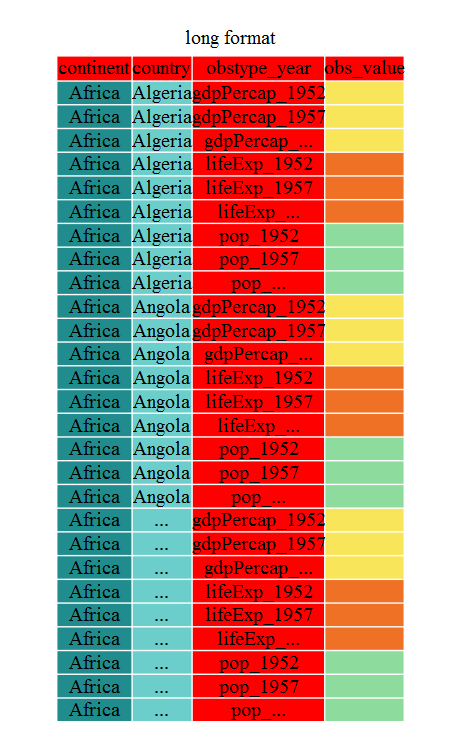
Now obstype_year actually contains 2 pieces of
information, the observation type
(pop,lifeExp, or gdpPercap) and
the year. We can use the separate() function
to split the character strings into multiple variables
R
gap_long <- gap_long %>% separate(obstype_year, into = c('obs_type', 'year'), sep = "_")
gap_long$year <- as.integer(gap_long$year)
R
gap_long %>% group_by(continent, obs_type) %>%
   summarize(means=mean(obs_values))
OUTPUT
`summarise()` has grouped output by 'continent'. You can override using the
`.groups` argument.
OUTPUT
# A tibble: 15 × 3
# Groups:   continent [5]
   continent obs_type       means
   <chr>     <chr>          <dbl>
 1 Africa    gdpPercap     2194.
 2 Africa    lifeExp         48.9
 3 Africa    pop        9916003.
 4 Americas  gdpPercap     7136.
 5 Americas  lifeExp         64.7
 6 Americas  pop       24504795.
 7 Asia      gdpPercap     7902.
 8 Asia      lifeExp         60.1
 9 Asia      pop       77038722.
10 Europe    gdpPercap    14469.
11 Europe    lifeExp         71.9
12 Europe    pop       17169765.
13 Oceania   gdpPercap    18622.
14 Oceania   lifeExp         74.3
15 Oceania   pop        8874672.
From long to intermediate format with pivot_wider()
It is always good to check work. So, let’s use the second
pivot function, pivot_wider(), to ‘widen’ our
observation variables back out. pivot_wider() is the
opposite of pivot_longer(), making a dataset wider by
increasing the number of columns and decreasing the number of rows. We
can use pivot_wider() to pivot or reshape our
gap_long to the original intermediate format or the widest
format. Let’s start with the intermediate format.
The pivot_wider() function takes names_from
and values_from arguments.
To names_from we supply the column name whose contents
will be pivoted into new output columns in the widened data frame. The
corresponding values will be added from the column named in the
values_from argument.
R
gap_normal <- gap_long %>%
  pivot_wider(names_from = obs_type, values_from = obs_values)
dim(gap_normal)
OUTPUT
[1] 1704 6R
dim(gapminder)
OUTPUT
[1] 1704 6R
names(gap_normal)
OUTPUT
[1] "continent" "country" "year" "gdpPercap" "lifeExp" "pop" R
names(gapminder)
OUTPUT
[1] "country" "year" "pop" "continent" "lifeExp" "gdpPercap"Now we’ve got an intermediate data frame gap_normal with
the same dimensions as the original gapminder, but the
order of the variables is different. Let’s fix that before checking if
they are all.equal().
R
gap_normal <- gap_normal[, names(gapminder)]
all.equal(gap_normal, gapminder)
OUTPUT
[1] "Attributes: < Component \"class\": Lengths (3, 1) differ (string compare on first 1) >"
[2] "Attributes: < Component \"class\": 1 string mismatch >"
[3] "Component \"country\": 1704 string mismatches"
[4] "Component \"pop\": Mean relative difference: 1.634504"
[5] "Component \"continent\": 1212 string mismatches"
[6] "Component \"lifeExp\": Mean relative difference: 0.203822"
[7] "Component \"gdpPercap\": Mean relative difference: 1.162302"
R
head(gap_normal)
OUTPUT
# A tibble: 6 × 6
  country  year      pop continent lifeExp gdpPercap
  <chr>   <int>    <dbl> <chr>       <dbl>     <dbl>
1 Algeria  1952  9279525 Africa       43.1     2449.
2 Algeria  1957 10270856 Africa       45.7     3014.
3 Algeria  1962 11000948 Africa       48.3     2551.
4 Algeria  1967 12760499 Africa       51.4     3247.
5 Algeria  1972 14760787 Africa       54.5     4183.
6 Algeria  1977 17152804 Africa       58.0     4910.
R
head(gapminder)
OUTPUT
      country year      pop continent lifeExp gdpPercap
1 Afghanistan 1952  8425333      Asia  28.801  779.4453
2 Afghanistan 1957  9240934      Asia  30.332  820.8530
3 Afghanistan 1962 10267083      Asia  31.997  853.1007
4 Afghanistan 1967 11537966      Asia  34.020  836.1971
5 Afghanistan 1972 13079460      Asia  36.088  739.9811
6 Afghanistan 1977 14880372      Asia  38.438  786.1134
We’re almost there, the original was sorted by country,
then year.
R
gap_normal <- gap_normal %>% arrange(country, year)
all.equal(gap_normal, gapminder)
OUTPUT
[1] "Attributes: < Component \"class\": Lengths (3, 1) differ (string compare on first 1) >"
[2] "Attributes: < Component \"class\": 1 string mismatch >"
That’s great! We’ve gone from the longest format back to the intermediate and we didn’t introduce any errors in our code.
Now let’s convert the long all the way back to the wide. In the wide
format, we will keep country and continent as ID variables and pivot the
observations across the 3 metrics
(pop,lifeExp,gdpPercap) and time
(year). First we need to create appropriate labels for all
our new variables (time*metric combinations) and we also need to unify
our ID variables to simplify the process of defining
gap_wide.
R
gap_temp <- gap_long %>% unite(var_ID, continent, country, sep = "_")
str(gap_temp)
OUTPUT
tibble [5,112 × 4] (S3: tbl_df/tbl/data.frame)
 $ var_ID    : chr [1:5112] "Africa_Algeria" "Africa_Algeria" "Africa_Algeria" "Africa_Algeria" ...
 $ obs_type  : chr [1:5112] "gdpPercap" "gdpPercap" "gdpPercap" "gdpPercap" ...
 $ year      : int [1:5112] 1952 1957 1962 1967 1972 1977 1982 1987 1992 1997 ...
 $ obs_values: num [1:5112] 2449 3014 2551 3247 4183 ...
R
gap_temp <- gap_long %>%
    unite(ID_var, continent, country, sep = "_") %>%
    unite(var_names, obs_type, year, sep = "_")
str(gap_temp)
OUTPUT
tibble [5,112 × 3] (S3: tbl_df/tbl/data.frame)
 $ ID_var    : chr [1:5112] "Africa_Algeria" "Africa_Algeria" "Africa_Algeria" "Africa_Algeria" ...
 $ var_names : chr [1:5112] "gdpPercap_1952" "gdpPercap_1957" "gdpPercap_1962" "gdpPercap_1967" ...
 $ obs_values: num [1:5112] 2449 3014 2551 3247 4183 ...
Using unite() we now have a single ID variable which is
a combination of continent,country,and we have
defined variable names. We’re now ready to pipe in
pivot_wider()
R
gap_wide_new <- gap_long %>%
  unite(ID_var, continent, country, sep = "_") %>%
  unite(var_names, obs_type, year, sep = "_") %>%
  pivot_wider(names_from = var_names, values_from = obs_values)
str(gap_wide_new)
OUTPUT
tibble [142 × 37] (S3: tbl_df/tbl/data.frame)
 $ ID_var        : chr [1:142] "Africa_Algeria" "Africa_Angola" "Africa_Benin" "Africa_Botswana" ...
 $ gdpPercap_1952: num [1:142] 2449 3521 1063 851 543 ...
 $ gdpPercap_1957: num [1:142] 3014 3828 960 918 617 ...
 $ gdpPercap_1962: num [1:142] 2551 4269 949 984 723 ...
 $ gdpPercap_1967: num [1:142] 3247 5523 1036 1215 795 ...
 $ gdpPercap_1972: num [1:142] 4183 5473 1086 2264 855 ...
 $ gdpPercap_1977: num [1:142] 4910 3009 1029 3215 743 ...
 $ gdpPercap_1982: num [1:142] 5745 2757 1278 4551 807 ...
 $ gdpPercap_1987: num [1:142] 5681 2430 1226 6206 912 ...
 $ gdpPercap_1992: num [1:142] 5023 2628 1191 7954 932 ...
 $ gdpPercap_1997: num [1:142] 4797 2277 1233 8647 946 ...
 $ gdpPercap_2002: num [1:142] 5288 2773 1373 11004 1038 ...
 $ gdpPercap_2007: num [1:142] 6223 4797 1441 12570 1217 ...
 $ lifeExp_1952  : num [1:142] 43.1 30 38.2 47.6 32 ...
 $ lifeExp_1957  : num [1:142] 45.7 32 40.4 49.6 34.9 ...
 $ lifeExp_1962  : num [1:142] 48.3 34 42.6 51.5 37.8 ...
 $ lifeExp_1967  : num [1:142] 51.4 36 44.9 53.3 40.7 ...
 $ lifeExp_1972  : num [1:142] 54.5 37.9 47 56 43.6 ...
 $ lifeExp_1977  : num [1:142] 58 39.5 49.2 59.3 46.1 ...
 $ lifeExp_1982  : num [1:142] 61.4 39.9 50.9 61.5 48.1 ...
 $ lifeExp_1987  : num [1:142] 65.8 39.9 52.3 63.6 49.6 ...
 $ lifeExp_1992  : num [1:142] 67.7 40.6 53.9 62.7 50.3 ...
 $ lifeExp_1997  : num [1:142] 69.2 41 54.8 52.6 50.3 ...
 $ lifeExp_2002  : num [1:142] 71 41 54.4 46.6 50.6 ...
 $ lifeExp_2007  : num [1:142] 72.3 42.7 56.7 50.7 52.3 ...
 $ pop_1952      : num [1:142] 9279525 4232095 1738315 442308 4469979 ...
 $ pop_1957      : num [1:142] 10270856 4561361 1925173 474639 4713416 ...
 $ pop_1962      : num [1:142] 11000948 4826015 2151895 512764 4919632 ...
 $ pop_1967      : num [1:142] 12760499 5247469 2427334 553541 5127935 ...
 $ pop_1972      : num [1:142] 14760787 5894858 2761407 619351 5433886 ...
 $ pop_1977      : num [1:142] 17152804 6162675 3168267 781472 5889574 ...
 $ pop_1982      : num [1:142] 20033753 7016384 3641603 970347 6634596 ...
 $ pop_1987      : num [1:142] 23254956 7874230 4243788 1151184 7586551 ...
 $ pop_1992      : num [1:142] 26298373 8735988 4981671 1342614 8878303 ...
 $ pop_1997      : num [1:142] 29072015 9875024 6066080 1536536 10352843 ...
 $ pop_2002      : num [1:142] 31287142 10866106 7026113 1630347 12251209 ...
$ pop_2007 : num [1:142] 33333216 12420476 8078314 1639131 14326203 ...R
gap_ludicrously_wide <- gap_long %>%
   unite(var_names, obs_type, year, country, sep = "_") %>%
   pivot_wider(names_from = var_names, values_from = obs_values)
Now we have a great ‘wide’ format data frame, but the
ID_var could be more usable, let’s separate it into 2
variables with separate()
R
gap_wide_betterID <- separate(gap_wide_new, ID_var, c("continent", "country"), sep="_")
gap_wide_betterID <- gap_long %>%
    unite(ID_var, continent, country, sep = "_") %>%
    unite(var_names, obs_type, year, sep = "_") %>%
    pivot_wider(names_from = var_names, values_from = obs_values) %>%
    separate(ID_var, c("continent","country"), sep = "_")
str(gap_wide_betterID)
OUTPUT
tibble [142 × 38] (S3: tbl_df/tbl/data.frame)
 $ continent     : chr [1:142] "Africa" "Africa" "Africa" "Africa" ...
 $ country       : chr [1:142] "Algeria" "Angola" "Benin" "Botswana" ...
 $ gdpPercap_1952: num [1:142] 2449 3521 1063 851 543 ...
 $ gdpPercap_1957: num [1:142] 3014 3828 960 918 617 ...
 $ gdpPercap_1962: num [1:142] 2551 4269 949 984 723 ...
 $ gdpPercap_1967: num [1:142] 3247 5523 1036 1215 795 ...
 $ gdpPercap_1972: num [1:142] 4183 5473 1086 2264 855 ...
 $ gdpPercap_1977: num [1:142] 4910 3009 1029 3215 743 ...
 $ gdpPercap_1982: num [1:142] 5745 2757 1278 4551 807 ...
 $ gdpPercap_1987: num [1:142] 5681 2430 1226 6206 912 ...
 $ gdpPercap_1992: num [1:142] 5023 2628 1191 7954 932 ...
 $ gdpPercap_1997: num [1:142] 4797 2277 1233 8647 946 ...
 $ gdpPercap_2002: num [1:142] 5288 2773 1373 11004 1038 ...
 $ gdpPercap_2007: num [1:142] 6223 4797 1441 12570 1217 ...
 $ lifeExp_1952  : num [1:142] 43.1 30 38.2 47.6 32 ...
 $ lifeExp_1957  : num [1:142] 45.7 32 40.4 49.6 34.9 ...
 $ lifeExp_1962  : num [1:142] 48.3 34 42.6 51.5 37.8 ...
 $ lifeExp_1967  : num [1:142] 51.4 36 44.9 53.3 40.7 ...
 $ lifeExp_1972  : num [1:142] 54.5 37.9 47 56 43.6 ...
 $ lifeExp_1977  : num [1:142] 58 39.5 49.2 59.3 46.1 ...
 $ lifeExp_1982  : num [1:142] 61.4 39.9 50.9 61.5 48.1 ...
 $ lifeExp_1987  : num [1:142] 65.8 39.9 52.3 63.6 49.6 ...
 $ lifeExp_1992  : num [1:142] 67.7 40.6 53.9 62.7 50.3 ...
 $ lifeExp_1997  : num [1:142] 69.2 41 54.8 52.6 50.3 ...
 $ lifeExp_2002  : num [1:142] 71 41 54.4 46.6 50.6 ...
 $ lifeExp_2007  : num [1:142] 72.3 42.7 56.7 50.7 52.3 ...
 $ pop_1952      : num [1:142] 9279525 4232095 1738315 442308 4469979 ...
 $ pop_1957      : num [1:142] 10270856 4561361 1925173 474639 4713416 ...
 $ pop_1962      : num [1:142] 11000948 4826015 2151895 512764 4919632 ...
 $ pop_1967      : num [1:142] 12760499 5247469 2427334 553541 5127935 ...
 $ pop_1972      : num [1:142] 14760787 5894858 2761407 619351 5433886 ...
 $ pop_1977      : num [1:142] 17152804 6162675 3168267 781472 5889574 ...
 $ pop_1982      : num [1:142] 20033753 7016384 3641603 970347 6634596 ...
 $ pop_1987      : num [1:142] 23254956 7874230 4243788 1151184 7586551 ...
 $ pop_1992      : num [1:142] 26298373 8735988 4981671 1342614 8878303 ...
 $ pop_1997      : num [1:142] 29072015 9875024 6066080 1536536 10352843 ...
 $ pop_2002      : num [1:142] 31287142 10866106 7026113 1630347 12251209 ...
 $ pop_2007      : num [1:142] 33333216 12420476 8078314 1639131 14326203 ...
R
all.equal(gap_wide, gap_wide_betterID)
OUTPUT
[1] "Attributes: < Component \"class\": Lengths (1, 3) differ (string compare on first 1) >"
[2] "Attributes: < Component \"class\": 1 string mismatch >"
There and back again!
Other great resources
- R for Data Science (online book)
- Data Wrangling Cheat sheet (pdf file)
- Introduction to tidyr (online documentation)
- Data wrangling with R and RStudio (online video)