
Instructor's Guide for Databases and SQL
Opening
In the late 1920s and early 1930s, William Dyer, Frank Pabodie, and Valentina Roerich led expeditions to the Pole of Inaccessibility in the South Pacific, and then onward to Antarctica. Two years ago, Gina Geographer discovered their expedition journals in a storage locker at Miskatonic University. She has scanned and OCR'd the data they contain, and wants to store that information in a way that will make search and analysis easy.
Gina basically has three options: text files, a spreadsheet, or a database. Text files are easiest to create, and work well with version control, but she would then have to build all her search and analysis herself. Spreadsheets are good for doing simple analysis, but as she found in her last project, they don't handle large or complex data sets very well. She would therefore like to put her data in a database, and this chapter will show her how.
As many scientists have found out the hard way, if collecting data is the first 90% of the work, managing it is the other 90%. In this chapter, we'll see how to use a database to store and analyze field observations. The techniques we will explore apply directly to other kinds of databases as well, and as we'll see, knowing how to get information out of a database is essential to figuring out how to put data in.
Instructors
- Relational databases are not as widely used in science as in business, but they are still a common way to store large data sets with complex structure. Even when the data itself isn't in a database, the metadata could be: for example, meteorological data might be stored in files on disk, but data about when and where observations were made, data ranges, and so on could be in a database to make it easier for scientists to find what they want to.
- The first few sections (up to Ordering Results) usually go very quickly. The pace usually slows down a bit when null values and aggregation are discussed, mostly because learners have a lot of details to keep straight by this point. Things really slow down during the discussion of joins, but this is the key idea in the whole lesson: important ideas like primary keys and referential integrity only make sense once learners have seen how they're used in joins. It's worth going over things a couple of times if necessary (with lots of examples).
- The final three sections are independent of each other, and can be dropped if time is short. Of the three, people seem to care most about how to add data (which only takes a few minutes to demonstrate), and how to use databases from inside "real" programs. The material on transactions is more abstract than the rest, and should be omitted if web programming isn't being taught. Overall, this material takes three hours to present assuming that a short exercise is done with each topic.
- It isn't necessary to cover sets and dictionaries before this material, but if that has been discussed, it's helpful to point out that a relational table is a generalized dictionary.
- Simple calculations are actually easier to do in a spreadsheet, the advantages of using a database become clear as soon as filtering and joins are needed. Instructors may therefore want to show a spreadsheet with the information from the four database tables consolidated into a single sheet, and demonstrate what's needed in both systems to answer questions like, "What was the average radiation reading in 1931?"
-
Some learners may have heard that NoSQL databases
(i.e., ones that don't use the relational model)
are the next big thing,
and ask why we're not teaching those.
The answers are:
- Relational databases are far more widely used than NoSQL databases.
- We have far more experience with relational databases than with any other kind, so we have a better idea of what to teach and how to teach it.
- NoSQL databases are as different from each other as they are from relational databases. Until a leader emerges, it isn't clear which NoSQL database we should teach.
- This discussion is a useful companion to that of vectorization in the lesson on numerical computing: in both cases, the key point is to describe what to do, and let the computer figure out how to do it.
Selecting
Objectives
- Explain the difference between a table, a database, and a database manager.
- Explain the difference between a field and a record.
- Select specific fields from specific tables, and display them in a specific order.
Duration: 15 minutes (not including time required to download database file and connect to it).
Lesson
A relational database is a way to store and manipulate information that is arranged as tables. Each table has columns (also known as fields) which describe the data, and rows (also known as records) which contain the data.
When we are using a spreadsheet, we put formulas into cells to calculate new values based on old ones. When we are using a database, we send commands (usually called queries) to a database manager: a program that manipulates the database for us. The database manager does whatever lookups and calculations the query specifies, returning the results in a tabular form that we can then use as a starting point for further queries.
Under the Hood
Every database manager—Oracle, IBM DB2, PostgreSQL, MySQL, Microsoft Access, and SQLite—stores data in a different way, so a database created with one cannot be used directly by another. However, every database manager can import and export data in a variety of formats, so it is possible to move information from one to another.
Queries are written in a language called SQL, which stands for "Structured Query Language". SQL provides hundreds of different ways to analyze and recombine data; we will only look at a handful, but that handful accounts for most of what scientists do.
Figure 1 shows a simple database that stores some of the data Gina extracted from the logs of those long-ago expeditions. It contains four tables:
| Table | Purpose |
|---|---|
Person |
People who took readings. |
Site |
Locations of observation sites. |
Visited |
When readings were taken at specific sites. |
Survey |
The actual measurement values. |
|
|
|||||||||||||||||||||||||||||||||||||||||||||||||||||||||||||||||||||||||||||||||||||||||||||||||||||||||||||||||
|
||||||||||||||||||||||||||||||||||||||||||||||||||||||||||||||||||||||||||||||||||||||||||||||||||||||||||||||||||
|
||||||||||||||||||||||||||||||||||||||||||||||||||||||||||||||||||||||||||||||||||||||||||||||||||||||||||||||||||
Notice that three entries—one in the Visited table,
and two in the Survey table—are shown as NULL.
We'll return to these values later.
For now,
let's write an SQL query that displays scientists' names.
We do this using the SQL command select,
giving it the names of the columns we want and the table we want them from.
Our query and its output look like this:
sqlite> select family, personal from Person;
| Dyer | William |
| Pabodie | Frank |
| Lake | Anderson |
| Roerich | Valentina |
| Danforth | Frank |
The semi-colon at the end of the query tells the database manager that the query is complete and ready to run. If we enter the query without the semi-colon, or press 'enter' part-way through the query, the SQLite interpreter will give us a different prompt to show us that it's waiting for more input:
sqlite> select family, personal
   ...> from Person
   ...> ;
| Dyer | William |
| Pabodie | Frank |
| Lake | Anderson |
| Roerich | Valentina |
| Danforth | Frank |
From now on, we won't bother to display the prompt(s) with our commands.
Case and Consistency
We have written our command and the column names in lower case, and the table name in title case, but we could use any mix: SQL is case insensitive, so we could write them all in upper case, or even like this:
SeLeCt famILY, PERSonal frOM PERson;
But please don't: large SQL queries are hard enough to read without the extra cognitive load of random capitalization.
Displaying Results
Exactly how the database displays the query's results depends on what kind of interface we are using. If we are running SQLite directly from the shell, its default output looks like this:
Dyer|William Pabodie|Frank Lake|Anderson Roerich|Valentina Danforth|FrankIf we are using a graphical interface, such as the SQLite Manager plugin for Firefox or the database extension for the IPython Notebook, our output will be displayed graphically (Figure 2 and Figure 3). We'll use a simple table-based display in these notes.


Going back to our query, it's important to understand that the rows and columns in a database table aren't actually stored in any particular order. They will always be displayed in some order, but we can control that in various ways. For example, we could swap the columns in the output by writing our query as:
select personal, family from Person; |
|
| William | Dyer |
| Frank | Pabodie |
| Anderson | Lake |
| Valentina | Roerich |
| Frank | Danforth |
or even repeat columns:
select ident, ident, ident from Person; |
||
| dyer | dyer | dyer |
| pb | pb | pb |
| lake | lake | lake |
| roe | roe | roe |
| danforth | danforth | danforth |
We will see ways to rearrange the rows later.
As a shortcut, we can select all of the columns in a table
using the wildcard *:
select * from Person; |
||
| dyer | William | Dyer |
| pb | Frank | Pabodie |
| lake | Anderson | Lake |
| roe | Valentina | Roerich |
| danforth | Frank | Danforth |
Key Points
- A relational database stores information in tables with fields and records.
- A database manager is a program that manipulates a database.
- The commands or queries given to a database manager are usually written in a specialized language called SQL.
- SQL is case insensitive.
- The rows and columns of a database table aren't stored in any particular order.
- Use
select fields from tableto get all the values for specific fields from a single table. - Use
select * from tableto select everything from a table.
Challenges
Write a query that selects only site names from the
Sitetable.Many people format queries as:
SELECT personal, family FROM person;
or as:
select Personal, Family from PERSON;
what style do you find easiest to read, and why?
Removing Duplicates
Objectives
- Write queries that only display distinct results once.
Lesson
Data is often redundant,
so queries often return redundant information.
For example,
if we select the quantitites that have been measured
from the survey table,
we get this:
select quant from Survey; |
| rad |
| sal |
| rad |
| sal |
| rad |
| sal |
| temp |
| rad |
| sal |
| temp |
| rad |
| temp |
| sal |
| rad |
| sal |
| temp |
| sal |
| rad |
| sal |
| sal |
| rad |
We can eliminate the redundant output
to make the result more readable
by adding the distinct keyword
to our query:
select distinct quant from Survey; |
| rad |
| sal |
| temp |
If we select more than one column—for example, both the survey site ID and the quantity measured—then the distinct pairs of values are returned:
select distinct taken, quant from Survey; |
|
| 619 | rad |
| 619 | sal |
| 622 | rad |
| 622 | sal |
| 734 | rad |
| 734 | sal |
| 734 | temp |
| 735 | rad |
| 735 | sal |
| 735 | temp |
| 751 | rad |
| 751 | temp |
| 751 | sal |
| 752 | rad |
| 752 | sal |
| 752 | temp |
| 837 | rad |
| 837 | sal |
| 844 | rad |
Notice in both cases that duplicates are removed even if they didn't appear to be adjacent in the database. Again, it's important to remember that rows aren't actually ordered: they're just displayed that way.
Key Points
- Use
distinctto eliminate duplicates from a query's output.
Challenges
Write a query that selects distinct dates from the
Sitetable.If you are using SQLite from the command line, you can run a single query by passing it to the interpreter right after the path to the database file:
$ sqlite3 survey.db 'select * from Person;'
dyer|William|Dyer
pb|Frank|Pabodie
lake|Anderson|Lake
roe|Valentina|Roerich
danforth|Frank|Danforth
Fill in the missing commands in the pipeline below so that the output contains no redundant values.
$ sqlite3 survey.db 'select person, quant from Survey;' | command 1 | command 2Do you think this is less efficient, just as efficient, or more efficient that using
distinctfor large data?
Filtering
Objectives
- Write queries that select records based on the values of their fields.
- Write queries that select records using combinations of several tests on their fields' values.
- Build up complex filtering criteria incrementally.
- Explain the logical order in which filtering by field value and displaying fields takes place.
Lesson
One of the most powerful features of a database is
the ability to filter data,
i.e.,
to select only those records that match certain criteria.
For example,
suppose we want to see when a particular site was visited.
We can select these records from the Visited table
by using a where clause in our query:
select * from Visited where site='DR-1'; |
||
| 619 | DR-1 | 1927-02-08 |
| 622 | DR-1 | 1927-02-10 |
| 844 | DR-1 | 1932-03-22 |
The database manager executes this query in two stages
(Figure 4).
First,
it checks at each row in the Visited table
to see which ones satisfy the where.
It then uses the column names following the select keyword
to determine what columns to display.
select * from Visited where site='DR-1';
|
select * from Visited where site='DR-1';
|
||||||||||||||||||||||||||||||||||||||||||||||
|
→ |
|
|||||||||||||||||||||||||||||||||||||||||||||
This processing order means that
we can filter records using where
based on values in columns that aren't then displayed:
select ident from Visited where site='DR-1'; |
| 619 |
| 622 |
| 844 |
We can use many other Boolean operators to filter our data. For example, we can ask for all information from the DR-1 site collected since 1930:
select * from Visited where (site='DR-1') and (dated>='1930-00-00'); |
||
| 844 | DR-1 | 1932-03-22 |
(The parentheses around the individual tests aren't strictly required, but they help make the query easier to read.)
Working With Dates
Most database managers have a special data type for dates. In fact, many have two: one for dates, such as "May 31, 1971", and one for durations, such as "31 days". SQLite doesn't: instead, it stores dates as either text (in the ISO-8601 standard format "YYYY-MM-DD HH:MM:SS.SSSS"), real numbers (the number of days since November 24, 4714 BCE), or integers (the number of seconds since midnight, January 1, 1970). If this sounds complicated, it is, but not nearly as complicated as figuring out historical dates in Sweden.
If we want to find out what measurements were taken by either Lake or Roerich,
we can combine the tests on their names using or:
select * from Survey where person='lake' or person='roe'; |
|||
| 734 | lake | sal | 0.05 |
| 751 | lake | sal | 0.1 |
| 752 | lake | rad | 2.19 |
| 752 | lake | sal | 0.09 |
| 752 | lake | temp | -16.0 |
| 752 | roe | sal | 41.6 |
| 837 | lake | rad | 1.46 |
| 837 | lake | sal | 0.21 |
| 837 | roe | sal | 22.5 |
| 844 | roe | rad | 11.25 |
Alternatively,
we can use in to see if a value is in a specific set:
select * from Survey where person in ('lake', 'roe');
|
|||
| 734 | lake | sal | 0.05 |
| 751 | lake | sal | 0.1 |
| 752 | lake | rad | 2.19 |
| 752 | lake | sal | 0.09 |
| 752 | lake | temp | -16.0 |
| 752 | roe | sal | 41.6 |
| 837 | lake | rad | 1.46 |
| 837 | lake | sal | 0.21 |
| 837 | roe | sal | 22.5 |
| 844 | roe | rad | 11.25 |
We can combine and with or,
but we need to be careful about which operator is executed first.
If we don't use parentheses,
we get this:
select * from Survey where quant='sal' and person='lake' or person='roe'; |
|||
| 734 | lake | sal | 0.05 |
| 751 | lake | sal | 0.1 |
| 752 | lake | sal | 0.09 |
| 752 | roe | sal | 41.6 |
| 837 | lake | sal | 0.21 |
| 837 | roe | sal | 22.5 |
| 844 | roe | rad | 11.25 |
which is salinity measurements by Lake, and any measurement by Roerich. We probably want this instead:
select * from Survey where quant='sal' and (person='lake' or person='roe'); |
|||
| 734 | lake | sal | 0.05 |
| 751 | lake | sal | 0.1 |
| 752 | lake | sal | 0.09 |
| 752 | roe | sal | 41.6 |
| 837 | lake | sal | 0.21 |
| 837 | roe | sal | 22.5 |
Finally,
we can use distinct with where
to give a second level of filtering:
select distinct person, quant from Survey where person='lake' or person='roe'; |
|
| lake | sal |
| lake | rad |
| lake | temp |
| roe | sal |
| roe | rad |
But remember:
distinct is applied to the values displayed in the chosen columns,
not to the entire rows as they are being processed.
Growing Queries
What we have just done is how most people "grow" their SQL queries. We started with something simple that did part of what we wanted, then added more clauses one by one, testing their effects as we went. This is a good strategy—in fact, for complex queries it's often the only strategy—but it depends on quick turnaround, and on us recognizing the right answer when we get it.
The best way to achieve quick turnaround is often to put a subset of data in a temporary database and run our queries against that, or to fill a small database with synthesized records. For example, instead of trying our queries against an actual database of 20 million Australians, we could run it against a sample of ten thousand, or write a small program to generate ten thousand random (but plausible) records and use that.
Key Points
- Use
where testin a query to filter records based on Boolean tests. - Use
andandorto combine tests. - Use
into check if a value is in a set. - Build up queries a bit at a time, and test them against small data sets.
Challenges
Gina wants to select all sites that lie within 30° of the equator. Her query is:
select * from Site where (lat > -30) or (lat < 30);
Explain why this is wrong, and rewrite the query so that it is correct.
Normalized salinity readings are supposed to be between 0.0 and 1.0. Write a query that selects all records from
Surveywith salinity values outside this range.The SQL test
column-name like patternis true if the value in the named column matches the pattern given; the character '%' can be used any number of times in the pattern to mean "match zero or more characters".Expression Value 'a' like 'a'True'a' like '%a'True'b' like '%a'False'alpha' like 'a%'True'alpha' like 'a%p%'True'beta' like 'a%p%'FalseThe expression
column-name not like patterninverts the test. Usinglike, write a query that finds all the records inVisitedthat aren't from sites labelled 'DR-something'.
Calculating New Values
Objectives
- Write queries that do arithmetic using the values in individual records.
Duration: 5 minutes.
Lesson
After carefully reading the expedition logs, Gina realizes that the radiation measurements they report may need to be corrected upward by 5%. Rather than modifying the stored data, she can do this calculation on the fly as part of her query:
select 1.05 * reading from Survey where quant='rad'; |
| 10.311 |
| 8.19 |
| 8.8305 |
| 7.581 |
| 4.5675 |
| 2.2995 |
| 1.533 |
| 11.8125 |
When we run the query,
the expression 1.05 * reading is evaluated for each row.
Expressions can use any of the fields,
all of usual arithmetic operators,
and a variety of common functions.
(Exactly which ones depends on which database manager is being used.)
For example,
we can convert temperature readings from Fahrenheit to Celsius
and round to two decimal places as follows:
select taken, round(5*(reading-32)/9, 2) from Survey where quant='temp'; |
|
| 734 | -29.72 |
| 735 | -32.22 |
| 751 | -28.06 |
| 752 | -26.67 |
We can also combine values from different fields,
for example by using the string concatenation operator ||:
select personal || ' ' || family from Person; |
| William Dyer |
| Frank Pabodie |
| Anderson Lake |
| Valentina Roerich |
| Frank Danforth |
A Note on Names
It may seem strange to use personal and family as field names
instead of first and last,
but it's a necessary first step toward handling cultural differences.
For example,
consider the following rules:
| Full Name | Alphabetized Under | Reason |
|---|---|---|
| Liu Xiaobo | Liu | Chinese family names come first |
| Leonardo da Vinci | Leonardo | "da Vinci" just means "from Vinci" |
| Catherine de Medici | Medici | family name |
| Jean de La Fontaine | La Fontaine | family name is "La Fontaine" |
| Juan Ponce de Leon | Ponce de Leon | full family name is "Ponce de Leon" |
| Gabriel Garcia Marquez | Garcia Marquez | double-barrelled Spanish surnames |
| Wernher von Braun | von or Braun | depending on whether he was in Germany or the US |
| Elizabeth Alexandra May Windsor | Elizabeth | monarchs alphabetize by the name under which they reigned |
| Thomas a Beckett | Thomas | and saints according to the names by which they were canonized |
Clearly, even a two-part division into "personal" and "family" isn't enough...
Key Points
- Use expressions as fields to calculate per-record values.
Challenges
After further reading, Gina realizes that Valentina Roerich was reporting salinity as percentages. Write a query that returns all of her salinity measurements from the
Surveytable with the values divided by 100.The
unionoperator combines the results of two queries:select * from Person where ident='dyer' union select * from Person where ident='roe';
dyer William Dyer roe Valentina Roerich Use
unionto create a consolidated list of salinity measurements in which Roerich's, and only Roerich's, have been corrected as described in the previous challenge. The output should be something like:619 0.13 622 0.09 734 0.05 751 0.1 752 0.09 752 0.416 837 0.21 837 0.225 The site identifiers in the
Visitedtable have two parts separated by a '-':select distinct site from Visited;
DR-1 DR-3 MSK-4 Some major site identifiers are two letters long and some are three. The "in string" function
instr(X, Y)returns the 1-based index of the first occurrence of string Y in string X, or 0 if Y does not exist in X. The substring functionsubstr(X, I)returns the substring of X starting at index I. Use these two functions to produce a list of unique major site identifiers. (For this data, the list should contain only "DR" and "MSK").Pabodie's journal notes that all his temperature measurements are in °F, but Lake's journal does not report whether he used °F or °C. How should Gina treat his measurements, and why?
Ordering Results
Objectives
- Write queries that order results according to fields' values.
- Write queries that order results according to calculated values.
- Explain why it is possible to sort records using the values of fields that are not displayed.
Duration: 5 minutes.
Lesson
As we mentioned earlier,
database records are not stored in any particular order.
This means that query results aren't necessarily sorted,
and even if they are,
we often want to sort them in a different way,
e.g., by the name of the project instead of by the name of the scientist.
We can do this in SQL by adding an order by clause to our query:
select reading from Survey where quant='rad' order by reading; |
| 1.46 |
| 2.19 |
| 4.35 |
| 7.22 |
| 7.8 |
| 8.41 |
| 9.82 |
| 11.25 |
By default,
results are sorted in ascending order
(i.e.,
from least to greatest).
We can sort in the opposite order using desc (for "descending"):
select reading from Survey where quant='rad' order by reading desc; |
| 11.25 |
| 9.82 |
| 8.41 |
| 7.8 |
| 7.22 |
| 4.35 |
| 2.19 |
| 1.46 |
(And if we want to make it clear that we're sorting in ascending order,
we can use asc instead of desc.)
We can also sort on several fields at once.
For example,
this query sorts results first in ascending order by taken,
and then in descending order by person
within each group of equal taken values:
select taken, person from Survey order by taken asc, person desc; |
|
| 619 | dyer |
| 619 | dyer |
| 622 | dyer |
| 622 | dyer |
| 734 | pb |
| 734 | pb |
| 734 | lake |
| 735 | pb |
| 735 | |
| 735 | |
| 751 | pb |
| 751 | pb |
| 751 | lake |
| 752 | roe |
| 752 | lake |
| 752 | lake |
| 752 | lake |
| 837 | roe |
| 837 | lake |
| 837 | lake |
| 844 | roe |
This is easier to understand if we also remove duplicates:
select distinct taken, person from Survey order by taken asc, person desc;
|
|
| 619 | dyer |
| 622 | dyer |
| 734 | pb |
| 734 | lake |
| 735 | pb |
| 735 | |
| 751 | pb |
| 751 | lake |
| 752 | roe |
| 752 | lake |
| 837 | roe |
| 837 | lake |
| 844 | roe |
Since sorting happens before columns are filtered, we can sort by a field that isn't actually displayed:
select reading from Survey where quant='rad' order by taken; |
| 9.82 |
| 7.8 |
| 8.41 |
| 7.22 |
| 4.35 |
| 2.19 |
| 1.46 |
| 11.25 |
We can also sort results by the value of an expression.
In SQLite,
for example,
the random function returns a pseudo-random integer
each time it is called
(i.e.,
once per record):
select random(), ident from Person; |
|
| -6309766557809954936 | dyer |
| -2098461436941487136 | pb |
| -2248225962969032314 | lake |
| 6062184424509295966 | roe |
| -1268956870222271271 | danforth |
So to randomize the order of our query results, e.g., when doing clinical trials, we can sort them by the value of this function:
select ident from Person order by random(); |
| danforth |
| pb |
| dyer |
| lake |
| roe |
select ident from Person order by random(); |
| roe |
| dyer |
| pb |
| lake |
| danforth |
Our query pipeline now has four stages (Figure 5):
- Select the rows that pass the
wherecriteria. - Sort them if required.
- Filter the columns according to the
selectcriteria. - Remove duplicates if required.

Key Points
- Use
order by(withascordesc) to order a query's results. - Use
randomto generate pseudo-random numbers.
Challenges
Create a list of sites identifiers and their distance from the equator in kilometers, sorted from furthest to closest. (A degree of latitude corresponds to 111.12 km.)
Gina needs a list of radiation measurements from all sites sorted by when they were taken. The query:
select * from Survey where quant='rad' order by taken;
produces the correct answer for the data used in our examples. Explain when and why it might produce the wrong answer.
Missing Data
Objectives
- Explain what databases use the special value
NULLto represent. - Explain why databases should not uses their own special values (like 9999 or "N/A") to represent missing or unknown data.
- Explain what atomic and aggregate calculations involving
NULLproduce, and why. - Write queries that include or exclude records containing
NULL.
Duration: 10-20 minutes (the latter figure includes time for an anecdote about what happens when you don't take nulls into account).
Lesson
Real-world data is never complete—there are always holes.
Databases represent these holes using special value called null.
null is not zero, False, or the empty string;
it is a one-of-a-kind value that means "nothing here".
Dealing with null requires a few special tricks
and some careful thinking.
To start,
let's have a look at the Visited table.
There are eight records,
but #752 doesn't have a date—or rather,
its date is null:
select * from Visited; |
||
| 619 | DR-1 | 1927-02-08 |
| 622 | DR-1 | 1927-02-10 |
| 734 | DR-3 | 1939-01-07 |
| 735 | DR-3 | 1930-01-12 |
| 751 | DR-3 | 1930-02-26 |
| 752 | DR-3 | |
| 837 | MS-4 | 1932-01-14 |
| 844 | DR-1 | 1932-03-22 |
Displaying Nulls
Different databases display nulls differently. Unfortunately, SQLite's default is to print nothing at all, which makes nulls easy to overlook (particularly if they're in the middle of a long row).
Null doesn't behave like other values. If we select the records that come before 1930:
select * from Visited where dated<'1930-00-00'; |
||
| 619 | DR-1 | 1927-02-08 |
| 622 | DR-1 | 1927-02-10 |
we get two results, and if we select the ones that come during or after 1930:
select * from Visited where dated>='1930-00-00'; |
||
| 734 | DR-3 | 1939-01-07 |
| 735 | DR-3 | 1930-01-12 |
| 751 | DR-3 | 1930-02-26 |
| 837 | MS-4 | 1932-01-14 |
| 844 | DR-1 | 1932-03-22 |
we get five,
but record #752 isn't in either set of results.
The reason is that
null<'1930-00-00'
is neither true nor false:
null means, "We don't know,"
and if we don't know the value on the left side of a comparison,
we don't know whether the comparison is true or false.
Since databases represent "don't know" as null,
the value of null<'1930-00-00'
is actually null.
null>='1930-00-00' is also null
because we can't answer to that question either.
And since the only records kept by a where
are those for which the test is true,
record #752 isn't included in either set of results.
Comparisons aren't the only operations that behave this way with nulls.
1+null is null,
5*null is null,
log(null) is null,
and so on.
In particular,
comparing things to null with = and != produces null:
select * from Visited where dated=NULL; |
select * from Visited where dated!=NULL; |
To check whether a value is null or not,
we must use a special test is null:
select * from Visited where dated is NULL; |
||
| 752 | DR-3 | |
or its inverse is not null:
select * from Visited where dated is not NULL; |
||
| 619 | DR-1 | 1927-02-08 |
| 622 | DR-1 | 1927-02-10 |
| 734 | DR-3 | 1939-01-07 |
| 735 | DR-3 | 1930-01-12 |
| 751 | DR-3 | 1930-02-26 |
| 837 | MS-4 | 1932-01-14 |
| 844 | DR-1 | 1932-03-22 |
Null values cause headaches wherever they appear. For example, suppose we want to find the all of salinity measurements that weren't taken by Dyer. It's natural to write the query like this:
select * from Survey where quant='sal' and person!='lake'; |
|||
| 619 | dyer | sal | 0.13 |
| 622 | dyer | sal | 0.09 |
| 752 | roe | sal | 41.6 |
| 837 | roe | sal | 22.5 |
but this query filters omits the records
where we don't know who took the measurement.
Once again,
the reason is that when person is null,
the != comparison produces null,
so the record isn't kept in our results.
If we want to keep these records
we need to add an explicit check:
select * from Survey where quant='sal' and (person!='lake' or person is null);
|
|||
| 619 | dyer | sal | 0.13 |
| 622 | dyer | sal | 0.09 |
| 735 | sal | 0.06 | |
| 752 | roe | sal | 41.6 |
| 837 | roe | sal | 22.5 |
We still have to decide whether this is the right thing to do or not. If we want to be absolutely sure that we aren't including any measurements by Lake in our results, we need to exclude all the records for which we don't know who did the work.
What Happens When You Forget
Several years ago, I was helping a group who were looking at the spread of drug-resistant tuberculosis (DRTB) in industrialized countries. In particular, they wanted to know if it was spreading faster among less affluent people.
We tackled the problem by combining two data sets. The first gave us skin and blood test results for DRTB along with patients' postal codes (the only identifying information we were allowed---we didn't even have gender). The second was Canadian census data that gave us median income per postal code. Since a PC is about 300-800 people, we felt justified in joining the first with the second to estimate incomes for people with positive and negative test results.
To our surprise, we didn't find a correlation between income and infection. We were just about to publish when someone spotted the mistake I'd made.
Question: Who doesn't have a postal code?
Answer: Homeless people.
When I did the join, I was throwing away homeless people, which introduced a statistically significant error in my results. But I couldn't just set the income of anyone without a postal code to zero, because our sample included another set of people without postal codes: 16-21 year olds whose addresses were suppressed because they had tested positive for sexually-transmitted diseases.
At this point the problem is no longer a database issue, but rather a question of statistics. The takeaway is, checking your queries when you're programming is as important as checking your samples when you're doing chemistry.
Key Points
- Use
nullin place of missing information. - Almost every operation involving
nullproducesnullas a result. - Test for nulls using
is nullandis not null.
Challenges
Write a query that sorts the records in
Visitedby date, omitting entries for which the date is not known (i.e., is null).What do you expect the query:
select * from Visited where dated in ('1927-02-08', null);to produce? What does it actually produce?
Some database designers prefer to use a sentinel value to mark missing data rather than
null. For example, they will use the date "0000-00-00" to mark a missing date, or -1.0 to mark a missing salinity or radiation reading (since actual readings cannot be negative). What does this simplify? What burdens or risks does it introduce?
Aggregation
Objectives
- Write queries that combine values from many records to create a single aggregate value.
- Write queries that put records into groups based on their values.
- Write queries that combine values group by group.
- Explain what is displayed for unaggregated fields when some fields are aggregated.
Lesson
Gina now wants to calculate ranges and averages for her data.
She knows how to select all of the dates from the Visited table:
select dated from Visited; |
| 1927-02-08 |
| 1927-02-10 |
| 1939-01-07 |
| 1930-01-12 |
| 1930-02-26 |
| 1932-01-14 |
| 1932-03-22 |
but to combine them,
she must use an aggregation function
such as min or max.
Each of these functions takes a set of records as input,
and produces a single record as output:
select min(dated) from Visited; |
| 1927-02-08 |
select max(dated) from Visited; |
| 1939-01-07 |
min and max are just two of
the aggregation functions built into SQL.
Three others are avg,
count,
and sum:
select avg(reading) from Survey where quant='sal'; |
| 7.20333333333 |
select count(reading) from Survey where quant='sal'; |
| 9 |
select sum(reading) from Survey where quant='sal'; |
| 64.83 |
We used count(reading) here,
but we could just as easily have counted quant
or any other field in the table,
or even used count(*),
since the function doesn't care about the values themselves,
just how many values there are.
SQL lets us do several aggregations at once. We can, for example, find the range of sensible salinity measurements:
select min(reading), max(reading) from Survey where quant='sal' and reading<=1.0; |
|
| 0.05 | 0.21 |
We can also combine aggregated results with raw results, although the output might surprise you:
select person, count(*) from Survey where quant='sal' and reading<=1.0; |
|
| lake | 7 |
Why does Lake's name appear rather than Roerich's or Dyer's? The answer is that when it has to aggregate a field, but isn't told how to, the database manager chooses an actual value from the input set. It might use the first one processed, the last one, or something else entirely.
Another important fact is that when there are no values to aggregate, aggregation's result is "don't know" rather than zero or some other arbitrary value:
select person, max(reading), sum(reading) from Survey where quant='missing'; |
||
One final important feature of aggregation functions is that
they are inconsistent with the rest of SQL in a very useful way.
If we add two values,
and one of them is null,
the result is null.
By extension,
if we use sum to add all the values in a set,
and any of those values are null,
the result should also be null.
It's much more useful,
though,
for aggregation functions to ignore null values
and only combine those that are non-null.
This behavior lets us write our queries as:
select min(dated) from Visited; |
| 1927-02-08 |
instead of always having to filter explicitly:
select min(dated) from Visited where dated is not null;
|
| 1927-02-08 |
Key Points
- Use aggregation functions like
sumandmaxto combine query results. - Use
countfunction to count the number of results. - If some fields are aggregated and others are not, the database manager chooses an arbitrary result for the unaggregated field.
- Most aggregation functions skip nulls when combining values.
Challenges
How many temperature readings did Frank Pabodie record, and what was their average value?
The average of a set of values is the sum of the values divided by the number of values. Does this mean that the
avgfunction returns 2.0 or 3.0 when given the values 1.0,null, and 5.0?Gina wants to calculate the difference between each individual radiation reading and the average of all the radiation readings. She writes the query:
select reading-avg(reading) from Survey where quant='rad';
What does this actually produce, and why?
The function
group_concat(field, separator)concatenates all the values in a field using the specified separator character (or ',' if the separator isn't specified). Use this to produce a one-line list of scientists' names, such as:William Dyer, Frank Pabodie, Anderson Lake, Valentina Roerich, Frank Danforth
Can you find a way to order the list by surname?
Grouping
Objectives
- Group results to be aggregated separately.
- Explain when grouping occurs in the processing pipeline.
Duration: 10 minutes.
Lesson
Aggregating all records at once doesn't always make sense. For example, suppose Gina suspects that there is a systematic bias in her data, and that some scientists' radiation readings are higher than others. We know that this doesn't work:
select person, count(reading), round(avg(reading), 2) from Survey where quant='rad'; |
||
| roe | 8 | 6.56 |
because the database manager selects a single arbitrary scientist's name rather than aggregating separately for each scientist. Since there are only five scientists, she could write five queries of the form:
select person, count(reading), round(avg(reading), 2) from Survey where quant='rad' and person='dyer'; |
||
| dyer | 2 | 8.81 |
but this would be tedious, and if she ever had a data set with fifty or five hundred scientists, the chances of her getting all of those queries right is small.
What we need to do is
tell the database manager to aggregate the hours for each scientist separately
using a group by clause:
select person, count(reading), round(avg(reading), 2) from Survey where quant='rad' group by person; |
||
| dyer | 2 | 8.81 |
| lake | 2 | 1.82 |
| pb | 3 | 6.66 |
| roe | 1 | 11.25 |
group by does exactly what its name implies:
groups all the records with the same value for the specified field together
so that aggregation can process each batch separately.
Since all the records in each batch have the same value for person,
it no longer matters that the database manager
is picking an arbitrary one to display
alongside the aggregated reading values
(Figure 6).

Just as we can sort by multiple criteria at once,
we can also group by multiple criteria.
To get the average reading by scientist and quantity measured,
for example,
we just add another field to the group by clause:
select person, quant, count(reading), round(avg(reading), 2) from Survey group by person, quant; |
|||
| sal | 1 | 0.06 | |
| temp | 1 | -26.0 | |
| dyer | rad | 2 | 8.81 |
| dyer | sal | 2 | 0.11 |
| lake | rad | 2 | 1.82 |
| lake | sal | 4 | 0.11 |
| lake | temp | 1 | -16.0 |
| pb | rad | 3 | 6.66 |
| pb | temp | 2 | -20.0 |
| roe | rad | 1 | 11.25 |
| roe | sal | 2 | 32.05 |
Note that we have added person to the list of fields displayed,
since the results wouldn't make much sense otherwise.
Let's go one step further and remove all the entries where we don't know who took the measurement:
select person, quant, count(reading), round(avg(reading), 2) from Survey where person is not null group by person, quant order by person, quant; |
|||
| dyer | rad | 2 | 8.81 |
| dyer | sal | 2 | 0.11 |
| lake | rad | 2 | 1.82 |
| lake | sal | 4 | 0.11 |
| lake | temp | 1 | -16.0 |
| pb | rad | 3 | 6.66 |
| pb | temp | 2 | -20.0 |
| roe | rad | 1 | 11.25 |
| roe | sal | 2 | 32.05 |
Looking more closely, this query:
-
selected records from the
Surveytable where thepersonfield was not null; -
grouped those records into subsets
so that the
personandquantvalues in each subset were the same; -
ordered those subsets first by
person, and then within each sub-group byquant; and -
counted the number of records in each subset,
calculated the average
readingin each, and chose apersonandquantvalue from each (it doesn't matter which ones, since they're all equal).
Our query processing pipeline now looks like Figure 7.

Key Points
- Use
group byto group values for separate aggregation.
Challenges
Write a single query that finds the earliest and latest date that each site was visited.
Show the records produced by each stage of Figure 7 for the following query:
select   min(reading), max(reading) from Survey
where    taken in (734, 735)
and      quant='temp'
group by taken, quant;
How can the query below be simplified without changing its result?
select   min(reading), max(reading) from Survey
where    taken in (734, 735)
and      quant='temp'
group by taken, quant;
Combining Data
Objectives
- Explain what primary keys and foreign keys are.
- Write queries that combine information from two or more tables by matching keys.
- Write queries using aliases for table names.
- Explain why the
tablename.fieldnamenotation is needed when tables are joined. - Explain the logical sequence of operations that occurs when two or more tables are joined.
Duration: 20 minutes (including time to walk through one small example step by step).
Lesson
In order to submit her data to a web site that aggregates historical meteorological data, Gina needs to format it as:
| latitude | longitude | date | quantity | reading |
However,
her latitudes and longitudes are in the Site table,
while the dates of measurements are in the Visited table
and the readings themselves are in the Survey table.
She needs to combine these tables somehow.
The SQL command to do this is join.
To see how it works,
let's start by joining the Site and Visited tables:
select * from Site join Visited; |
|||||
| DR-1 | -49.85 | -128.57 | 619 | DR-1 | 1927-02-08 |
| DR-1 | -49.85 | -128.57 | 622 | DR-1 | 1927-02-10 |
| DR-1 | -49.85 | -128.57 | 734 | DR-3 | 1939-01-07 |
| DR-1 | -49.85 | -128.57 | 735 | DR-3 | 1930-01-12 |
| DR-1 | -49.85 | -128.57 | 751 | DR-3 | 1930-02-26 |
| DR-1 | -49.85 | -128.57 | 752 | DR-3 | |
| DR-1 | -49.85 | -128.57 | 837 | MS-4 | 1932-01-14 |
| DR-1 | -49.85 | -128.57 | 844 | DR-1 | 1932-03-22 |
| DR-3 | -47.15 | -126.72 | 619 | DR-1 | 1927-02-08 |
| DR-3 | -47.15 | -126.72 | 622 | DR-1 | 1927-02-10 |
| DR-3 | -47.15 | -126.72 | 734 | DR-3 | 1939-01-07 |
| DR-3 | -47.15 | -126.72 | 735 | DR-3 | 1930-01-12 |
| DR-3 | -47.15 | -126.72 | 751 | DR-3 | 1930-02-26 |
| DR-3 | -47.15 | -126.72 | 752 | DR-3 | |
| DR-3 | -47.15 | -126.72 | 837 | MS-4 | 1932-01-14 |
| DR-3 | -47.15 | -126.72 | 844 | DR-1 | 1932-03-22 |
| MS-4 | -48.87 | -123.4 | 619 | DR-1 | 1927-02-08 |
| MS-4 | -48.87 | -123.4 | 622 | DR-1 | 1927-02-10 |
| MS-4 | -48.87 | -123.4 | 734 | DR-3 | 1939-01-07 |
| MS-4 | -48.87 | -123.4 | 735 | DR-3 | 1930-01-12 |
| MS-4 | -48.87 | -123.4 | 751 | DR-3 | 1930-02-26 |
| MS-4 | -48.87 | -123.4 | 752 | DR-3 | |
| MS-4 | -48.87 | -123.4 | 837 | MS-4 | 1932-01-14 |
| MS-4 | -48.87 | -123.4 | 844 | DR-1 | 1932-03-22 |
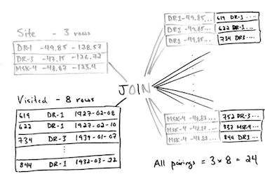
join creates
the cross product
of two tables,
i.e.,
it joins each record of one with each record of the other
to give all possible combinations (Figure 8).
Since there are three records in Site
and eight in Visited,
the join's output has 24 records.
And since each table has three fields,
the output has six fields.
What the join hasn't done is figure out if the records being joined have anything to do with each other. It has no way of knowing whether they do or not until we tell it how. To do that, we add a clause specifying that we're only interested in combinations that have the same site name:
select * from Site join Visited on Site.name=Visited.site;
|
|||||
| DR-1 | -49.85 | -128.57 | 619 | DR-1 | 1927-02-08 |
| DR-1 | -49.85 | -128.57 | 622 | DR-1 | 1927-02-10 |
| DR-1 | -49.85 | -128.57 | 844 | DR-1 | 1932-03-22 |
| DR-3 | -47.15 | -126.72 | 734 | DR-3 | 1939-01-07 |
| DR-3 | -47.15 | -126.72 | 735 | DR-3 | 1930-01-12 |
| DR-3 | -47.15 | -126.72 | 751 | DR-3 | 1930-02-26 |
| DR-3 | -47.15 | -126.72 | 752 | DR-3 | |
| MS-4 | -48.87 | -123.4 | 837 | MS-4 | 1932-01-14 |
on does the same job as where:
it only keeps records that pass some test.
(The difference between the two is that on filters records
as they're being created,
while where waits until the join is done
and then does the filtering.)
Once we add this to our query,
the database manager throws away records
that combined information about two different sites,
leaving us with just the ones we want.
Notice that we used table.field to specify field names
in the output of the join.
We do this because tables can have fields with the same name,
and we need to be specific which ones we're talking about.
For example,
if we joined the person and visited tables,
the result would inherit a field called ident
from each of the original tables.
We can now use the same dotted notation to select the three columns we actually want out of our join:
select Site.lat, Site.long, Visited.dated
from   Site join Visited
on     Site.name=Visited.site;
|
||
| -49.85 | -128.57 | 1927-02-08 |
| -49.85 | -128.57 | 1927-02-10 |
| -49.85 | -128.57 | 1932-03-22 |
| -47.15 | -126.72 | |
| -47.15 | -126.72 | 1930-01-12 |
| -47.15 | -126.72 | 1930-02-26 |
| -47.15 | -126.72 | 1939-01-07 |
| -48.87 | -123.4 | 1932-01-14 |
If joining two tables is good,
joining many tables must be better.
In fact,
we can join any number of tables
simply by adding more join clauses to our query,
and more on tests to filter out combinations of records
that don't make sense:
select Site.lat, Site.long, Visited.dated, Survey.quant, Survey.reading from Site join Visited join Survey on Site.name=Visited.site and Visited.ident=Survey.taken and Visited.dated is not null; |
||||
| -49.85 | -128.57 | 1927-02-08 | rad | 9.82 |
| -49.85 | -128.57 | 1927-02-08 | sal | 0.13 |
| -49.85 | -128.57 | 1927-02-10 | rad | 7.8 |
| -49.85 | -128.57 | 1927-02-10 | sal | 0.09 |
| -47.15 | -126.72 | 1939-01-07 | rad | 8.41 |
| -47.15 | -126.72 | 1939-01-07 | sal | 0.05 |
| -47.15 | -126.72 | 1939-01-07 | temp | -21.5 |
| -47.15 | -126.72 | 1930-01-12 | rad | 7.22 |
| -47.15 | -126.72 | 1930-01-12 | sal | 0.06 |
| -47.15 | -126.72 | 1930-01-12 | temp | -26.0 |
| -47.15 | -126.72 | 1930-02-26 | rad | 4.35 |
| -47.15 | -126.72 | 1930-02-26 | sal | 0.1 |
| -47.15 | -126.72 | 1930-02-26 | temp | -18.5 |
| -48.87 | -123.4 | 1932-01-14 | rad | 1.46 |
| -48.87 | -123.4 | 1932-01-14 | sal | 0.21 |
| -48.87 | -123.4 | 1932-01-14 | sal | 22.5 |
| -49.85 | -128.57 | 1932-03-22 | rad | 11.25 |
We can tell which records from Site, Visited, and Survey
correspond with each other
because those tables contain
primary keys
and foreign keys.
A primary key is a value,
or combination of values,
that uniquely identifies each record in a table.
A foreign key is a value (or combination of values) from one table
that identifies a unique record in another table.
Another way of saying this is that
a foreign key is the primary key of one table
that appears in some other table.
In our database,
Person.ident is the primary key in the Person table,
while Survey.person is a foreign key
relating the Survey table's entries
to entries in Person.
Most database designers believe that every table should have a well-defined primary key. They also believe that this key should be separate from the data itself, so that if we ever need to change the data, we only need to make one change in one place. One easy way to do this is to create an arbitrary, unique ID for each record as we add it to the database. This is actually very common: those IDs have names like "student numbers" and "patient numbers", and they almost always turn out to have originally been a unique record identifier in some database system or other. As the query below demonstrates, SQLite automatically numbers records as they're added to tables, and we can use those record numbers in queries:
select rowid, * from Person; |
|||
| 1 | dyer | William | Dyer |
| 2 | pb | Frank | Pabodie |
| 3 | lake | Anderson | Lake |
| 4 | roe | Valentina | Roerich |
| 5 | danforth | Frank | Danforth |
Key Points
- Use
jointo create all possible combinations of records from two or more tables. - Use
join tables on testto keep only those combinations that pass some test. - Use
table.fieldto specify a particular field of a particular table. - Every record in a table should be uniquely identified by the value of its primary key.
Challenges
Write a query that lists all radiation readings from the DR-1 site.
Write a query that lists all sites visited by people named "Frank".
Describe in your own words what the following query produces:
select Site.name from Site join Visited
on Site.lat<-49.0 and Site.name=Visited.site and Visited.dated>='1932-00-00';
Why does the
Persontable have anidentfield? Why do we not just use scientists' names in theSurveytable?Why does the table
Siteexist? Why didn't Gina just record latitudes and longitudes directly in theVisitedandSurveytables?
Creating and Modifying Tables
Objectives
- Write queries that create database tables with fields of common types.
- Write queries that specify the primary and foreign key relationships of tables.
- Write queries that specify whether field values must be unique and/or are allowed to be
null. - Write queries that erase database tables.
- Write queries that add records to database tables.
- Write queries that delete specific records from tables.
- Explain what referential integrity is, and how a database can become inconsistent as data is changed.
Duration: 10-15 minutes.
Lesson
So far we have only looked at how to get information out of a database, both because that is more frequent than adding information, and because most other operations only make sense once queries are understood. If we want to create and modify data, we need to know two other pairs of commands.
The first pair are create table and drop table.
While they are written as two words,
they are actually single commands.
The first one creates a new table;
its arguments are the names and types of the table's columns.
For example,
the following statements create the four tables in our survey database:
create table Person(ident text, personal text, family text);
create table Site(name text, lat real, long real);
create table Visited(ident integer, site text, dated text);
create table Survey(taken integer, person text, quant real, reading real);
We can get rid of one of our tables using:
drop table Survey;
Be very careful when doing this: most databases have some support for undoing changes, but it's better not to have to rely on it.
Different database systems support different data types for table columns, but most provide the following:
integer
|
A signed integer. |
real
|
A floating point value. |
text
|
A string. |
blob
|
Any "binary large object" such as an image or audio file. |
most databases also support Booleans and date/time values; SQLite uses the integers 0 and 1 for the former, and represents the latter as discussed earlier. An increasing number of databases also support geographic data types, such as latitude and longitude. Keeping track of what particular systems do or do not offer, and what names they give different data types, is an unending portability headache.
When we create a table,
we can specify several kinds of constraints on its columns.
For example,
a better definition for the Survey table would be:
create table Survey(
        taken   integer not null, -- where reading taken
        person  text,             -- may not know who took it
        quant   real not null,    -- the quantity measured
        reading real not null,    -- the actual reading
        primary key(taken, quant),
        foreign key(taken) references Visited(ident),
        foreign key(person) references Person(ident)
);
Once again, exactly what constraints are avialable and what they're called depends on which database manager we are using.
Once tables have been created,
we can add and remove records using our other pair of commands,
insert and delete.
The simplest form of insert statement lists values in order:
insert into Site values('DR-1', -49.85, -128.57);
insert into Site values('DR-3', -47.15, -126.72);
insert into Site values('MSK-4', -48.87, -123.40);
We can also insert values into one table directly from another:
create table JustLatLong(lat text, long TEXT);
insert into JustLatLong select lat, long from site;
Deleting records can be a bit trickier,
because we have to ensure that the database remains internally consistent.
If all we care about is a single table,
we can use the DELETE command with a WHERE clause
that matches the records we want to discard.
For example,
once we realize that Frank Danforth didn't take any measurements,
we can remove him from the Person table like this:
delete from Person where ident = "danforth";
But what if we removed Anderson Lake instead?
Our Survey table would still contain seven records
of measurements he'd taken:
select count(*) from Survey where person='lake'; |
| 7 |
That's never supposed to happen:
Survey.person is a foreign key into the Person table,
and all our queries assume there will be a row in the latter
matching every value in the former.
This problem is called referential integrity:
we need to ensure that all references between tables can always be resolved correctly.
One way to do this is to delete all the records
that use 'lake' as a foreign key
before deleting the record that uses it as a primary key.
If our database manager supports it,
we can automate this
using cascading delete.
However,
this technique is outside the scope of this chapter.
Other Ways to Do It
Many applications use a hybrid storage model instead of putting everything into a database: the actual data (such as astronomical images) is stored in files, while the database stores the files' names, their modification dates, the region of the sky they cover, their spectral characteristics, and so on. This is also how most music player software is built: the database inside the application keeps track of the MP3 files, but the files themselves live on disk.
Key Points
- Use
create table name(...)to create a table. - Use
drop table nameto erase a table. - Specify field names and types when creating tables.
- Specify
primary key,foreign key,not null, and other constraints when creating tables. - Use
insert into table values(...)to add records to a table. - Use
delete from table where testto erase records from a table. - Maintain referential integrity when creating or deleting information.
Challenges
Write an SQL statement to replace all uses of
nullinSurvey.personwith the string'unknown'.One of Gina's colleagues has sent her a CSV file containing temperature readings by Robert Olmstead, which is formatted like this:
Taken,Temp
619,-21.5
622,-15.5
Write a small Python program that reads this file in and prints out the SQL
insertstatements needed to add these records to the survey database. Note: you will need to add an entry for Olmstead to thePersontable. If you are testing your program repeatedly, you may want to investigate SQL'sinsert or replacecommand.SQLite has several administrative commands that aren't part of the SQL standard. One of them is
.dump, which prints the SQL commands needed to re-create the database. Another is.load, which reads a file created by.dumpand restores the database. A colleague of yours thinks that storing dump files (which are text) in version control is a good way to track and manage changes to the database. What are the pros and cons of this approach?
Transactions
Objectives
- Explain what a race condition is.
- Explain why database operations sometimes have to be placed ina transaction to ensure correct behavior.
- Explain what it means to commit a transaction.
Duration: 15 minutes.
Lesson
Suppose we have another table in our database that shows which pieces of equipment have been borrowed by which scientists:
select * from Equipment; |
|
| dyer | CX-211 oscilloscope |
| pb | Greenworth balance |
| lake | Cavorite damping plates |
(We should actually give each piece of equipment a unique ID, and use that ID here instead of the full name, just as we created a separate table for scientists earlier in this chapter, but we will bend the rules for now.) If William Dyer gives the oscilloscope to Valentina Roerich, we need to execute two statements to update this table:
delete from Equipment where person="dyer" and thing="CX-211 oscilloscope";
insert into Equipment values("roe", "CX-211 oscilloscope");
This is all fine—unless our program happens to crash
between the first statement and the second.
If that happens,
the Equipment table won't have a record for the oscilloscope at all.
Such a crash may seem unlikely,
but remember:
if a computer can do two billion operations per second,
that means there are two billion opportunities every second for something to go wrong.
And if our operations take a long time to complete—as they will
when we are working with large datasets,
or when the database is being heavily used—the odds of failure increase.
What we really want is a way to ensure that every operation is ACID: atomic (i.e. indivisible), consistent, isolated, and durable. The precise meanings of these terms doesn't matter; what does is the notion that every logical operation on the database should either run to completion as if nothing else was going on at the same time, or fail without having any effect at all.
The tool we use to ensure that this happens is called a transaction. Here's how we should actually write the statements to move the oscilloscope from one person to another:
begin transaction;
delete from Equipment where person="dyer" and thing="CX-211 oscilloscope";
insert into Equipment values("roe", "CX-211 oscilloscope");
end transaction;
The database manager treats everything in the transaction as one large statement. If anything goes wrong inside, then none of the changes made in the transaction will actually be written to the database—it will be as if the transaction had never happened. Changes are only stored permanently when we commit them at the end of the transaction.
Transactions and Commits
We first used the term "transaction" in our discussion of version control. That's not a coincidence: behind the scenes, tools like Subversion are using many of the same algorithms as database managers to ensure that either everything happens consistently or nothing happens at all. We use the term "commit" for the same reason: just as our changes to local files aren't written back to the version control repository until we commit them, our (apparent) changes to a database aren't written to disk until we say so.
Transactions serve another purpose as well.
Suppose there is another table in the database called Exposure
that records the number of days each scientist was exposed to
higher-than-normal levels of radiation:
select * from Exposure; |
|
| pb | 4 |
| dyer | 1 |
| lake | 5 |
After going through the journal entries for 1932, Gina wants to add two days to Lake's count:
update Exposure set days = days + 2 where person='lake';
However, her labmate has been doing through the journal entries for 1933 to help Gina meet a paper deadline. At the same moment as Gina runs her command, her labmate runs this to add one more day to Lake's exposure:
update Exposure set days = days + 1 where person='lake';
After both operations have completed, the database should show that Lake was exposed for eight days (the original five, plus two from Gina, plus one from her labmate). However, there is a small chance that it won't. To see why, let's break the two queries into their respective read and write steps and place them side by side:
X = read Exposure('lake', __) |
Y = read Exposure('lake', __) |
write Exposure('lake', X+2) |
write Exposure('lake', Y+1) |
The database can only actually do one thing at once, so it must put these four operations into some sequential order. That order has to respect the original order within each column, but the database can interleave the two columns any way it wants. If it orders them like this:
X = read Exposure('lake', __) |
X is 5 |
write Exposure('lake', X+2) |
database contains 7 |
Y = read Exposure('lake', __) |
Y is 7 |
write Exposure('lake', Y+1) |
database contains 8 |
then all is well. But what if it interleaves the operations like this:
X = read Exposure('lake', __) |
X is 5 |
Y = read Exposure('lake', __) |
Y is 5 |
write Exposure('lake', X+2) |
database contains 7 |
write Exposure('lake', Y+1) |
database contains 6 |
This ordering puts the initial value, 5, into both X and Y.
It then writes 7 back to the database (the third statement),
and then overwrites that with 6,
since Y holds 5.
This is called a race condition, since the final result depends on a race between the two operations. Race conditions are part of what makes programming large systems with many components a nightmare: they are difficult to spot in advance (since they are caused by the interactions between components, rather than by anything in any one of those components), and can be almost impossible to debug (since they usually occur intermittently and infrequently).
Transactions come to our rescue once again. If Gina and her labmate put their statements in transactions, the database will act as if it executed all of one and then all of the other. Whether or not it actually does this is up to whoever wrote the database manager: modern databases use very sophisticated algorithms to determine which operations actually have to be run sequentially, and which can safely be run in parallel to improve performance. The key thing is that every transaction will appear to have had the entire database to itself.
Key Points
- Place operations in a transaction to ensure that they appear to be atomic, consistent, isolated, and durable.
Challenges
A friend of yours manages a database of aerial photographs. New records are added all the time, but existing records are never modified or updated. Your friend claims that because of this, he doesn't need to put his queries in transactions. Is he right or wrong, and why?
Programming with Databases
Objectives
- Write a Python program that queries a database and processes the results.
- Explain what an SQL injection attack is.
- Write a program that safely interpolates values into queries.
Duration: 20 minutes.
Lesson
To end this chapter, let's have a look at how to access a database from a general-purpose programming language like Python. Other languages use almost exactly the same model: library and function names may differ, but the concepts are the same.
Here's a short Python program that selects latitudes and longitudes
from an SQLite database stored in a file called survey.db:
import sqlite3
connection = sqlite3.connect("survey.db")
cursor = connection.cursor()
cursor.execute("select site.lat, site.long from site;")
results = cursor.fetchall()
for r in results:
    print r
cursor.close()
connection.close()
The program starts by importing the sqlite3 library.
If we were connecting to MySQL, DB2, or some other database,
we would import a different library,
but all of them provide the same functions,
so that the rest of our program does not have to change
(at least, not much)
if we switch from one database to another.
Line 2 establishes a connection to the database. Since we're using SQLite, all we need to specify is the name of the database file. Other systems may require us to provide a username and password as well. Line 3 then uses this connection to create a cursor; just like the cursor in an editor, its role is to keep track of where we are in the database.
On line 4, we use that cursor to ask the database to execute a query for us.
The query is written in SQL,
and passed to cursor.execute as a string.
It's our job to make sure that SQL is properly formatted;
if it isn't,
or if something goes wrong when it is being executed,
the database will report an error.
The database returns the results of the query to us
in response to the cursor.fetchall call on line 5.
This result is a list with one entry for each record in the result set;
if we loop over that list (line 6) and print those list entries (line 7),
we can see that each one is a tuple
with one element for each field we asked for.
Finally, lines 8 and 9 close our cursor and our connection, since the database can only keep a limited number of these open at one time. Since establishing a connection takes time, though, we shouldn't open a connection, do one operation, then close the connection, only to reopen it a few microseconds later to do another operation. Instead, it's normal to create one connection that stays open for the lifetime of the program.
What Are The u's For?
You may have noticed that each of the strings in our output has a lower-case 'u' in front of it. That is Python's way of telling us that the string is stored in Unicode.
Queries in real applications will often depend on values provided by users. For example, a program might take a user ID as a command-line parameter and display the user's full name:
import sys
import sqlite3

query = "select personal, family from Person where ident='%s';"
user_id = sys.argv[1]

connection = sqlite3.connect("survey.db")
cursor = connection.cursor()

cursor.execute(query % user_id)
results = cursor.fetchall()
print results[0][0], results[0][1]

cursor.close()
connection.close()
The variable query holds the statement we want to execute
with a %s format string where we want to insert
the ID of the person we're looking up.
It seems simple enough,
but what happens if someone gives the program this input?
dyer"; drop table Survey; select "
It looks like there's garbage after the name of the project, but it is very carefully chosen garbage. If we insert this string into our query, the result is:
select personal, family from Person where ident='dyer'; drop table Survey; select '';
Whoops: if we execute this, it will erase one of the tables in our database.
This technique is called SQL injection, and it has been used to attack thousands of programs over the years. In particular, many web sites that take data from users insert values directly into queries without checking them carefully first.
Since a villain might try to smuggle commands into our queries in many different ways, the safest way to deal with this threat is to replace characters like quotes with their escaped equivalents, so that we can safely put whatever the user gives us inside a string. We can do this by using a prepared statement instead of formatting our statements as strings. Here's what our example program looks like if we do this:
import sys
import sqlite3

query = "select personal, family from Person where ident=?;"
user_id = sys.argv[1]

connection = sqlite3.connect("survey.db")
cursor = connection.cursor()

cursor.execute(query, [user_id])
results = cursor.fetchall()
print results[0][0], results[0][1]

cursor.close()
connection.close()
The key changes are in the query string and the execute call.
Instead of formatting the query ourselves,
we put question marks in the query template where we want to insert values.
When we call execute,
we provide a list
that contains as many values as there are question marks in the query.
The library matches values to question marks in order,
and translates any special characters in the values
into their escaped equivalents
so that they are safe to use.
Key Points
- Most applications that use databases embed SQL in a general-purpose programming language.
- Database libraries use connections and cursors to manage interactions.
- Programs can fetch all results at once, or a few results at a time.
- If queries are constructed dynamically using input from users, malicious users may be able to inject their own commands into the queries.
- Dynamically-constructed queries can use SQL's native formatting to safeguard against such attacks.
Challenges
Write a Python program that creates a new database in a file called
original.dbcontaining a single table calledPressure, with a single field calledreading, and inserts 100,000 random numbers between 10.0 and 25.0. How long does it take this program to run? How long does it take to run a program that simply writes those random numbers to a file?Write a Python program that creates a new database called
backup.dbwith the same structure asoriginal.dband copies all the values greater than 20.0 fromoriginal.dbtobackup.db. Which is faster: filtering values in the query, or reading everything into memory and filtering in Python?
Summary
There are many things databases can't do, or can't do well (which is why we have general-purpose programming languages like Python). However, they are still the best tool available for managing many kinds of complex, structured data. Thousands of programmer-years have gone into their design and implementation so that they can handle very large datasets—terabytes or more—quickly and reliably. Queries allow for great flexibility in how you are able to analyze your data, which makes databases a good choice when you are exploring data.